概率图模型9：贝叶斯网络

概率图模型最棒的性质就是因子分解与独立性之间的内在联系。
现在我们将要探讨，这种内在联系是如何在有向图（也就是贝叶斯网络）中体现的。

1. d-separation

d分离的概念我们在之前的博客中讲过，你可以到《概率图模型4：贝叶斯网络》中详细阅读。这里我们只给出更容易让人理解的表达方式。

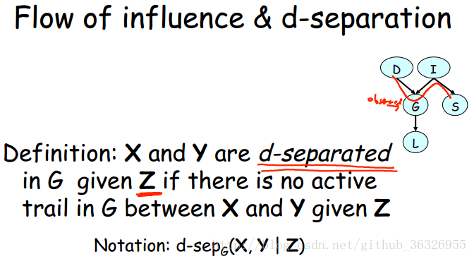
So we talked about the notion of flow of
influence in a probabilistic graphical
model where we have for example the
notion of an active trail that goes
through as up through I, down through G
and up through D, if for example we have
the G is observed, that is in Z.
And that gave us an intuition about which
what problistic influence might flow.
We can now turn this notion on its head
and ask the question well what happens
when we tell you that there are no active
trails on the graph that is influence
can’t flow.
So we’re going to make that notion formal
using the notion of d-separation.
And we’re going to say that X and Y are
deseparated in a graph G given a set of
observation Z if there’s a lack of trail
between them.
And the intuition that would like to
demonstrate in this context is that this
notion of influence can’t flow
corresponds much more formally to the
rigorous notion of conditional
independence in the graph.
So let’s actually prove that that’s in
fact the case.
So the theorem that we’d like to state
that if P factorizes over the graph,
then P factorized is over G.
And we have a deseparation property that
holds in the graph.
So X and Y are deseparated in the graph.
There’s no active trails between them.
Then P satisfies these conditional
statements,
X is independent of Y given Z.
So deseparation implies independence.
If, the, probability distribution
factorizes over G.
So, we’re now going to prove the theorem
in its full glory.
We’re going to prove it by example
because that example really just, it
really does illustrate the main points of
the derivation.
So, the assumption is that here is our
graph G, and here is the factorization of
the distribution.
So, according to the chain rule, of
Bayesian networks.
And this is a factorization that we’ve
seen before.
And so now we’d like to prove that a
d-separation statement follows from this
from this deriva-, from this assumption.
And, and the d-separation statement that
we’d like to prove follows as an
independence.
Is one that says that d is independent of
S.
First, let’s convince ourselves that D
and S are in fact d-separated in this
graph.
And so we see that there is only one
possible trail between d and s in this
graph.
It goes.
That instance g is not observed in this
case, and neither is l.
We have the, the trail is not activated
and so they, the two are, the two nodes
are de-separated and so, we’d like to
prove that this independence holds.
So what is the prob, the joint
probability distribution, of D and S?
Well it’s the sum over this join
distribution over here.
Marginalizing out the three variables
that are now D and S so GL and I so we
have the sum over GL and I of this big
product that’s defined by the tin roll.
And as we’ve previously seen when we have
a summation like that one of the things
that we can do is we can push in
summations into the product so long as we
don’t push them through terms that
involve the variable.
So here for example we have we might have
a summation over L.
And we can push in that summation because
the only term that involves L is the
probability of L given G.
So if we push in the summations in this
way we end up with the following
expression and we see that we have this
summation over L here, a summation over G
and then finally the summation over I at
the very beginning.
And what do we know about the summation
over L of P of L given G?
We know that this, that this is a
probability distribution over L and
therefore.
It’s necessarily sums to one, because
we’re summing up over all of the possible
values of L.
Once this term is one, we can look at the
next term, which is this one.
And we can ask ourselves, well one is,
cancels out, so probability, what is the
sum over G of the probability of G given
D and I, and that too is one.
And by the time we’re done, we end up
with the following expression.
And the important thing to notice about
this expression is that this is phi one
of D and this is phi two, oops.
I two of S, and therefore because we
partitioned this joint distribution as a
product of two factors, we end up with
something that corresponds directly to
the definition of marginal dependence,
therefore proving that P satisfies this
independent statement.
Having convinced ourselves that
de-separation is an interesting notion,
let’s look at some other de-separation
statements that might hold in a graph.
So, one general statement that we can
show is that any node in the graph is
de-separated.
From it’s non-descendants given it’s
parents.
So let’s look at the variable letter.
And let’s see what non-descendants,
non-descendants it has that are not it’s
parents.
So it only has two descendants let’s mark
those in blue it’s this one and that one
and what are the non-descendants so these
are the descendants.
What about the non-descendants?
Well, here’s one non-descendant, here’s
another, another and another.
So, those are the four non-descendants in
the graph that are not parents.
So, now let’s convince ourselves that,
letter is de-separated from all of it’s
non-descendants given it’s parents and
let’s take just an arbitrary one of
those, let’s take S A T for example and
let’s see if we can find an active trail
from S A T to letter that is active given
the parents, which, in this case, is just
a variable grade.
Okay.
So what are, what’s one potential trail?
So we can go this way, up.
And then back down through water, but is
that trail active?
No its not active because Greg is
observed and so drop with blocks a trail
in fact it will block any trail that
comes in from the top.
So any trail into letter that comes in
through its parents grave is going to be
blocked by the fact that grade is
observed.
So that means we have to come in through
the bottom.
So let’s look at that.
So let’s look at the trail from s a t,
through job.
An up, again through letter, well is that
trail active, no.
The reason it’s not active is because
only great is observed, and job, since
it’s not, it can’t be a parent of, our
letter, because it’s a descendent, is
necasserily not observed and so neither
job nor happy, are observed and so we, we
can not activate, this V structure, over
here, can not be activated and so, trails
that come in from the bottom, don’t work
either.
And so we again this is a proof by a
demonstration but it shows again that
that.
It shows the general property in a very
simple way.
So that tells us by the theorem that we
proved on the previous slide that if P
factorizes over G, then we know that any
variable is indepedent.
Of it’s non-descendants given its
parents, which is a kind of nice
intuition when you think about it.
Because when we motivated the structure
of Bayesian networks we basically said
that what makes us pick the, the parents
for a node is the set of, of variables
that are the only ones that this variable
depends on.
So the parents of are the variables on
which depends directly.
And this gives a formal semantics to that
intuition.
That is we now have the variable is
depending only on its parents.
So, now that we’ve defined a set of
independencies that hold for any
distribution that factorizes over a
graph, we’re now going to define a
general notion, which is just a term for
this.
So we define d-separation in a graph G
and, and we showed that when you have the
d-separation property, that P satisfies
the corresponding independence statement.
And so now we can basically look at the
independencies that are implied by the
graph G.
So I of g which is the set of
indepedencies that are implicit in a
graph G are all of the independent
statements X is independent of Y given Z
that correspond to d-seperation
statements within the graph.
So this is the set of all indepedencies
that are derived from d-seperation
statements and those are the ones that
the graph implies hold for distribution P
as we just showed in the previous demo.
So, now we can give this a name.
We going to say that P if P satisfies all
the in-dependencies of G, then G is an
I-map of P, and I-map stands for
in-dependency map.
And the reason its an independancy map is
by looking at G it’s a map of
independancy as a hole in p.
That is it maps independancies that we
know to be true.
So let’s look at examples in imap, so
let’s look at two two distributions here
is one distribution p1.
And here is a second distribution, P2.
Now lets look at two possible graphs.
One is G1 that has D and I being separate
variables.
And the other, is G2 that has an edge
between D and I.
So what independencies does G1 apply?
What’s an I of G1?
Well I of G1.
Is the independence that says d is
independent of I, because there’s no
edges between them.
What’s I of g2?
One of, IT2 implies no independencies,
because, there are no, because D and I
are connected by an edge and there’s no
other independencies that can be implied,
and so, I of G2 is named B7.
So what does that tell us, let’s look at
the connection between these graphs and
these two distributions, is G1 an I map
of P1, well, if you look at P1, you can
convince yourself that P1, satisfies, D
is independent of I, J1 isn’t I map.
Fp1.
What about G, is G1 an I map of P2?
Well, if we look at P2, we can, again,
convince ourselves by examination that P2
doesn’t satisfy.
D is independent of i.
So the answer is no.
this, g1 is not an I map for p2.
What about the other direction, what
about g2?
Well, G two has no independent
assumptions, and so it satisfies, and so,
it both P one and P two satisfy the empty
set of independence assumptions.
As it happens P one also satisfies
additional independence assumptions but
the definitions of Imap didn’t require
that that G, that a graph exactly
represent the independents in, in in a
distribution, only that any independence
that’s implied by the graph holds for the
distribution, and so we have.
The G2 is actually an I-map for both P1
and P2.
So now we can restate the theorem that we
stated before.
Before we talked about the separation
properties so now we can just give it a
one concise statement.
We can say that if P factorizes over G,
that is if it’s representable of the
bayesian network over G, then G is an
IMAP for P, which means I can read from
G.
Independencies that hold in P.
Regardless of the perimeters.
That’s by knowing that P factorizes over
G.
Interestingly, the converse of this
theorem holds also.
So this version of the theorem says that
if g is an imap for p, than p factorizes
over g.
So what does that mean?
It means that if the graph, if the
distribution satisfies the independence
assumptions that are implicit in the
graph, then we can take that distribution
and represent it as a Bayesian network
over that graph.
So once again, let’s do a proof by
example.
So now here we have the little graph that
we’re going to use.
And and so now what do we know?
We’re going to write down the probability
of the join distribution over the, these
five random variables using this
expression.
Which is the chain rule for
probabilities.
Not the chain rule for Bayesian networks,
because.
We don’t know yet that this is
representable as a Bayesian network.
We’re going to write the chain rule for
probabilities.
And that has us, writing it as P of D
times P of I given D.
Which, if you multiply the two together
using the definition of conditional
probability.
These two, together, give us the
probability of I, D.
If we multiply that by G, given IND.
Then we end up with the probability of G,
I, D.
And so on, we can construct this
telescoping product.
And altogether we, by multiplying all
these conditional probabilities we have a
we have a, the def-,
we can reconstruct the original joint
probability distribution.
Great,
now what?
So we haven’t used any notions of
independence yet.
So where do we use that?
Well, we’re going to look at each one of
these terms.
And we’re going to see how we can
simplify it.
So P of D is already as simple as it
gets.
So now, let’s look at, the next term.
Which is probability of I given D.
And let’s look at this graph.
And we can see that I and D are non
descendants.
And we’re not conditioning on any parents
and so we have that in this graph as and
we’ve already shown this that I is
independent of D.
And so we can using one of the
definitions that we have of conditional
independence, we can erase this from the
right hand side of the conditioning bar
and just get P of I.
The next term is already in the form that
we want is so we don’t need to do
anything with it but now let’s look at
the probability of S given D, I and G.
So here we have the probability of a
variable S, given one of its parents I
and one of its non-descendants D and G.
And we know that S is independent of its
non-descendant given, non-descendants
given its parent I and so we can erase
both D and G and so end up with the
probability of S given I.
Finally, we have the last term,
probability of L, given D, I, G, and S.
And here again, we have the probability
of a variable L, given it’s parent G, and
a bunch of long descendants, so we can
again, erase the long descendants.
And so all together that gives us exactly
the expression that we wanted.
And so now, again, by example we proved
this we proved this independent, we
proved that from these independent
statements we can derive the fact that P
factorizes using the product rule for
base E networks.
To summarize, we have provided to
equivalent views of the graph structure.
The first is the graph as a
factorization, as a data structure that
tells us how the distribution P can be
broken up in to pieces.
So, in this case, the fact that G allows
P to be represented as a set of factors
or CPD’s over the network.
The second is the Imap view, the fact
that the definition that the, that the
structure of G and code independencies
that necessarily hold in P.
Now what we’ve shown is that each of
these actually implies the other.
Which means, if, that if we have a
distribution p that we know is
represented as a Bayesian network over a
certain graph, we can just look at the
graph, and let even delving into
parameters know certain independencies
that have to hold in the distribution P.
And independencies is a really valuable
thing because it’ll, it tells you
something about what influences what, and
if I observe something, what else might
change.
And that helps a lot in understanding the
structure of the distribution and
consequences of different types of
observations.

朴素贝叶斯

One subclass of Bayesian Networks is the
class called as Naive Bayes or sometimes
even more derogatory, Idiot Bayes.
As we’ll see Naive Bayes models are
called that way because they make
independence assumptions that indeed very
naive and orally simplistic.
And yet they provide an interesting point
on the tradeoff curve, be, of model
complexity that sometimes turns out to be
surprisingly useful.
So here is a naive base model.
the small is typically used for
classification that is taking an instance
where we have effectively observed a
bunch of features.
And in most cases, although not
necessarily, we’re assuming that all of
these features are observed for each of
the, for a given instance.
And our goal is to infer to which class
among a limited set of classes a
particular instance belongs.
So these are observed, these ones here
observed, and this one in general is
hidden.
Now if you look at the, assumptions made
by this model, this model makes the
assumption that every pair of features XI
and XJ are conditionally independent.
Given class so every xi and xj give us no
information.
One gives no information about the other
once the class variable is observed.
Which reduces this whole model into one
where we only have to encode individual
pairwise interactions between the class
variable and single features.
So if we look at the chain rule for
Bayesian networks, as applied in this
context, we see that we have a joined
distribution, P of C comma X one of the
XN, which can be written using a product
form as a prior over the class variable
C, and a product of the conditional
probabilities of each feature, given the
class.
To understand this model a little bit
better, it helps us to look at the ratio
between the probabilities of two
different classes, given a particular
observation.
That is a particular assignment X1 of the
Xn to the observed features.
So if we look at this ratio we can see
that it can be broken down as a product
of two terms.
The first is just the ratio of the prior
probabilities of the two classes.
So that’s the green term here and the
second is this blue term which of all the
ratios as it’s called.
That is the probability of seeing a
particular observation xi in the context
of one class, relative to the context of
the other class.
So let’s look at an application of the
naive base model in one of the places
where it’s actually very commonly used,
which is the context of text
classification.
So imagine that we’re trying to take a
document and figure out for that document
to which category it belongs.
We have some set of categories in mind.
So for example, is this a document about
pets, is it about finance, is it about
vacations?
We have some set of categories and we’d
like to assign a document to one of
those.
It turns out that one can use two
different naive based models for tackling
this problem.
The first of those is called the
Bernoulli naive Bayes model for text.
And it, it treats every word in a
dictionary so you open your dictionary,
and there’s sev, several, you know, ten,
maybe 10,000 words in that dictionary.
And so you have a random variable for
every one of those words, or at least the
ones that occur in the kind of document
that you’re, you’re interested in
thinking about, and for each word in the
dictionary, we have a binary random
variable, which is one.
If the word appears in the document.
And zero otherwise.
If we have say, five thousand words that
we’re interested in, and anything about
we would have five thousand of these
binary variables, and so the propability
associated, the CPD, associated with each
variable is, in this case the propability
that the word appears say the propability
that the cat, the word cat appears, given
the label of the document.
So, for example, if we had, two
categories, that we’re looking at right
now, say documents about finances versus
documents about, documents about pets,
you would expect that in a document about
pets the word cat is quite likely to
appear.
and so I’m only showing the probability
of cats appearing.
the probability of cats not appearing
would be 0.7.
the probability that dog appears might be
0.4, and, and so on.
Where as for document about finances,
we’re less likely to see the word cat and
dog that are more likely to have the
words buy and sell so the probability
that buy appears might be considerably
higher in this case.
So this is a Bernoulli naive based model
because first it, it its a Bernoulli
model because each of these is a binary
variable with subject to a Bernoulli
Distribution, so this is a Bernoulli
Distribution.
And its naive based because it makes very
strong independence assumptions that the
probability of one word appearing is
independent of sorry, the event of one
word appearing is independent of the
event of a different word appearing given
that we know the class.
And obviously that assumption is far too
strong to be represented in the reality,
but it turns out to be a not bad
approximation.
In terms of actual performance.
A second model for the same problem is
what’s called the multi-nomial naive base
model for text.
In this case, the variables that
represent the features are not the words
in the dictionary, but rather, words in
the document.
So here, N is the length of the document.
If you have a document that has 737
words, you’re going to have 737 random
variables.
And the value of each of these random
variables is the actual word.
That is in the first second up to the Nth
position in the document.
And so the, if you have say that same
dictionary of 5,000 possible words, this
is no longer a binary random variable,
but rather, one that has the values where
this is the size of a dictionary,
say 5,000.
Now this might seem like a very
complicated model, because the c, p, d
now needs to specify the probability
distribution over words in the dictionary
for every possible word.
Very possible position in the document.
So, we need to have a probability
distribution over the words and word in
position one and position two and in
position N.
But we’re going to address that by
assuming that these probability
distributions are all the same.
And so the probability distribution for
over words in position one is the same a,
as for words in position two, three and
so on.
Now this is a multi nomial naive base
model, because notice that the
parameterization, for each of these
words, is a multi nomial distribution.
So what we see here, is not the same as
what we saw in the previous slide, where
we had a bunch of binary random
variables.
Here this is a multi nomial which means
that all these entries sum to one.
And it’s a naive based model because it
makes, again, a strong independence
assumption, a different independence
assumption, in this case it makes the
assumption that the word in position one
is independent of the word in position
two given the class variable.
And once again, if you think about say
two word phrases that care common this
assumption is clearly overly strong and
yet it appears to be a good
approximation.
In a variety of practical applications
and most notably, in the case of of
natural, of this kind of document
classification where it’s still quite
commonly used.
So to summarize, naive beta actually
provides us with a very simple approach
for classification problems.
It’s computationally very efficient.
And, the models are easy to construct.
Whether by had or by machine learning
techniques.
It turns out to be a surprisingly effect
method in domains that have a large
number of weekly relevant features, such
as the textual lanes that we’ve talked
about.
On the other hand, the strong independent
assumptions that we talked about, the
conditional independence of different
features given the class, reduce the
performance of these models, especially
in cases when we have multiple, highly
correlated features.