Matlab神经网络十讲(2): Create Configuration & Train NeuralNet

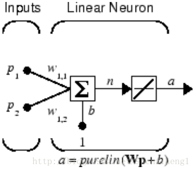
1. Create Neural Network Object

The easiest way to create a neural network is to use one of the network creation functions. To investigate how this is done, you can create a simple, two-layer feedforward network, using the command feedforwardnet (前馈神经网络）:

The dimensions section stores the overall structure of the network. Here you can see that there is one input to the network (although the one input can be a vector containing many elements), one network output, and two layers.

The connections section stores the connections between components of the network. For example, there is a bias connected to each layer, the input is connected to layer 1, and the output comes from layer 2. You can also see that layer 1 is connected to layer 2. (The rows of net.layerConnect represent the destination layer, and the columns represent the source layer. A one in this matrix indicates a connection, and a zero indicates no connection. For this example, there is a single one in element 2,1 of the matrix.)

The key subobjects of the network object are inputs, layers, outputs, biases, inputWeights, and layerWeights.View the layers subobject for the first layer with the command：

net.layers{1}

Neural Network Layer
           name: 'Hidden'
     dimensions: 10
    distanceFcn: (none)
  distanceParam: (none)
      distances: []
        initFcn: 'initnw'
    netInputFcn: 'netsum'
  netInputParam: (none)
      positions: []
          range: [10x2 double]
           size: 10
    topologyFcn: (none)
    transferFcn: 'tansig'
  transferParam: (none)
       userdata: (your custom info)

The number of neurons in a layer is given by its size property. In this case, the layer has 10 neurons, which is the default size for the feedforwardnet command. The net input function is netsum (summation) and the transfer function is the tansig. If you wanted to change the transfer function to logsig, for example, you could execute the
command:

net.layers{1}.transferFcn = 'logsig';

To view the layerWeights subobject for the weight between layer 1 and layer 2, use the command:

net.layerWeights{2,1}

Neural Network Weight
           delays: 0
          initFcn: (none)
       initConfig: .inputSize
            learn: true
         learnFcn: 'learngdm'
       learnParam: .lr, .mc
             size: [0 10]
        weightFcn: 'dotprod'
      weightParam: (none)
         userdata: (your custom info)

The weight function is dotprod, which represents standard matrix multiplication (dot product). Note that the size of this layer weight is 0-by-10. The reason that we have zero rows is because the network has not yet been configured for a particular data set. The number of output neurons is equal to the number of rows in your target vector. During
the configuration process, you will provide the network with example inputs and targets, and then the number of output neurons can be assigned.

functions:

adaptFcn: 'adaptwb'

adaptParam: (none) derivFcn: 'defaultderiv' divideFcn: 'dividerand' divideParam: .trainRatio, .valRatio, .testRatio divideMode: 'sample' initFcn: 'initlay' performFcn: 'mse' performParam: .regularization, .normalization plotFcns: {'plotperform', plottrainstate, ploterrhist, plotregression} plotParams: {1x4 cell array of 4 params} trainFcn: 'trainlm' trainParam: .showWindow, .showCommandLine, .show, .epochs, .time, .goal, .min_grad, .max_fail, .mu, .mu_dec, .mu_inc, .mu_max

methods:
       adapt: Learn while in continuous use
   configure: Configure inputs & outputs
      gensim: Generate Simulink model
        init: Initialize weights & biases
     perform: Calculate performance
         sim: Evaluate network outputs given inputs
       train: Train network with examples
        view: View diagram
 unconfigure: Unconfigure inputs & outputs

2.Configure Neural Network Inputs and Outputs

After a neural network has been created, it must be configured. The configuration step consists of examining input and target data, setting the network's input and output sizes to match the data, and choosing settings for processing inputs and outputs that will enable best network performance.
However, it can be done manually, by using the configuration function. For example, to configure the network you created previously to approximate a sine function, issue the following commands:

p = -2:.1:2;
t = sin(pi*p/2);
net1 = configure(net,p,t);

You have provided the network with an example set of inputs and targets (desired network outputs). With this information, the configure function can set the network
input and output sizes to match the data.

In addition to setting the appropriate dimensions for the weights, the configuration step alsodefines the settings for the processing of inputs and outputs.The input processing can be located in the inputssubobject:

net1.inputs{1}
   Neural Network Input
            name: 'Input'
  feedbackOutput: []
     processFcns: {'removeconstantrows', mapminmax}
   processParams: {1x2 cell array of 2 params}
 processSettings: {1x2 cell array of 2 settings}
  processedRange: [1x2 double]
   processedSize: 1
           range: [1x2 double]
            size: 1
        userdata: (your custom info)

Before the input is applied to the network, i t will be processed by two functions: removeconstantrows and mapminmax. These processing functions may have some processing parameters, which are contained in the subobject net1.inputs{1}.processParam. These have default values that you can override. The processing functions can also have configuration settings that are dependent on the sample data. These are contained in net1.inputs{1}.processSettings and are set during the configuration process. For example, the mapminmax processing function normalizes the data so that all inputs fall in the range [−1, 1]. Its configuration settings include the minimum and maximum values in the sample data, which it needs to perform the correct normalization. 

3.Understanding Neural Network Toolbox Data Structures

3.1 Simulation with Concurrent Inputs in a Static Network

The simplest situation for simulating a network occurs when the network to be simulated is static (has no feedback or delays). In this case, you need not be concerned about whether or not the input vectors occur in a particular time sequence, so you can treat the inputs as concurrent. In addition, the problem is made even simpler by assuming that
the network has only one input vector. Use the following network as an example.

set up this linear feedforward network:

net = linearlayer;
net.inputs{1}.size = 2;
net.layers{1}.dimensions = 1;

For simplicity, assign the weight matrix and bias to be W = [1 2] and b = [0].The commands for these assignments are:

net.IW{1,1} = [1 2];
net.b{1} = 0;

Suppose that the network simulation data set consists of Q = 4 Left.Concurrent vectors are presented to the network as a single matrix:

P = [1 2 2 3; 2 1 3 1];

We can now simulate the network: A = net(P) 

3.2 Simulation with Sequential Inputs in a Dynamic Network

When a network contains delays, the input to the network would normally be a sequence of input vectors that occur in a certain time order. To illustrate this case, the next figure shows a simple network that contains one delay.

The following commands create this network:

net = linearlayer([0 1]);
net.inputs{1}.size = 1;
net.layers{1}.dimensions = 1;
net.biasConnect = 0;

Assign the weight matrix to be W = [1 2]. The command is:

net.IW{1,1} = [1 2];

4. Neural Network Training Concepts

This topic describes two different styles of training. In incremental training(增量训练)the weights and biases of the network are updated each time an input is presented to the network. In batch training（批量训练） the weights and biases are only updated after all the inputs are presented.

4.1 Incremental Training with adapt

Incremental training can be applied to both static and dynamic networks, although it is more commonly used with dynamic networks, such as adaptive filters. 
4.1.1. Incremental Training of Static Networks
1. Suppose we want to train the network to create the linear function: T = 2*p1 + P2
   Then for the previous inputs,the targets would be t1=4;t2=5;t3=7;t4=7;
   For incremental training, you present the inputs and targets as sequences:

P = {[1;2] [2;1] [2;3] [3;1]};
T = {4 5 7 7};

2. First, set up the network with zero initial weights and biases. Also, set the initial learning rate to zero to show the effect of incremental training.

net = linearlayer(0,0);
net = configure(net,P,T);
net.IW{1,1} = [0 0];
net.b{1} = 0;

When you use the adapt function, if the inputs are presented as a cell array of sequential vectors, then the
weights are updated as each input is presented (incremental mode).

We are now ready to train the network incrementally:

[net,a,e,pf] = adapt(net,P,T);

The network outputs remain zero, because the learning rate is zero, and the weights are not updated. The errors are equal to the targets:

a = [0] [0] [0] [0]
e = [4] [5] [7] [7]

If we now set the learning rate to 0.1 you can see how the network is adjusted as each input is presented:

net.inputWeights{1,1}.learnParam.lr = 0.1;
net.biases{1,1}.learnParam.lr = 0.1;
[net,a,e,pf] = adapt(net,P,T);

a = [0] [2] [6] [5.8]
e = [4] [3] [1] [1.2]

The first output is the same as it was with zero learning rate, because no update is made until the first input is presented. The second output is different, because the weights have been updated. The weights continue to be modified as each error is computed. If the network is capable and the learning rate is set correctly, the error is eventually driven to zero.

4.1.2 Incremental Training with Dynamic Networks
略 大同小异；详细部分可以参考UserGuide。

4.2 Batch Training

Batch training, in which weights and biases are only updated after all the inputs and targets are presented, can be applied to both static and dynamic networks. 

4.2.1 Batch Training with Static Networks

Batch training can be done using either adapt or train, although train is generally the best option, because it typically has access to more efficient training algorithms.Incremental training is usually done with adapt; batch training is usually done with train.
For batch training of a static network with adapt, the input vectors must be placed in one matrix of concurrent vectors.

P = [1 2 2 3; 2 1 3 1];
T = [4 5 7 7];

Begin with the static network used in previous examples. The learning rate is set to 0.01.

net = linearlayer(0,0.01);
net = configure(net,P,T);
net.IW{1,1} = [0 0];
net.b{1} = 0;

When we call adapt, it invokes trains (the default adaption function for the linear network) and learnwh (the default learning function for the weights and biases). trains uses Widrow-Hoff learning.

[net,a,e,pf] = adapt(net,P,T);
a = 0 0 0 0
e = 4 5 7 7

Note that the outputs of the network are all zero, because the weights are not updated until all the training set has been presented. If we display the weights, we find:

net.IW{1,1}    ans = 0.4900 0.4100
net.b{1}       ans = 0.2300

Now perform the same batch training using train. Because the Widrow-Hoff rule can be used in incremental or batch mode, it can be invoked by adapt or train. (There are several algorithms that can only be used in batch mode (e.g., Levenberg-Marquardt), so these algorithms can only be invoked by train.)
Train it for only one epoch, because we used only one pass of adapt. The default training function for the linear network is trainb, and the default learning function for the weights and biases is learnwh, so we should get the same results obtained using adapt in the previous example, where the default adaption function was trains.

net.trainParam.epochs = 1;
net = train(net,P,T);

If we display the weights after one epoch of training, we find:

net.IW{1,1}    ans = 0.4900 0.4100
net.b{1}       ans = 0.2300

This is the same result as the batch mode training in adapt. With static networks, the adapt function can implement incremental or batch training, depending on the format of the input data. If the data is presented as a matrix of concurrent vectors, batch training occurs. If the data is presented as a sequence, incremental training occurs. 

对比实验：

net = linearlayer(0,0.01);
net = configure(net,P,T);
net.IW{1,1} = [0 0];
net.b{1} = 0;
net.trainParam.epochs = 1;
net = train(net,P,T);

net = linearlayer(0,0.01);
net = configure(net,P,T);
net.IW{1,1} = [0 0];
net.b{1} = 0;
net.trainParam.epochs = 100;
net = train(net,P,T);

4.2.2 Batch Training with Dynamic Networks

略，大同小异。

5. Training Feedback

The showWindow parameter allows you to specify whether a training window is visible when you train. The training window appears by default. Two other parameters,showCommandLine and show, determine whether command-line output is generated and the number of epochs between command-line feedback during training. For instance, followed code turns off the training window and gives you training status information every 35 epochs when the network is later trained with train:

net.trainParam.showWindow = false;
net.trainParam.showCommandLine = true;
net.trainParam.show= 35;

Sometimes it is convenient to disable all training displays. To do that, turn off both the training window and command-line feedback:

net.trainParam.showWindow = false;
net.trainParam.showCommandLine = false;

The training window appears automatically when you train. Use the nntraintool function to manually open and close the training window.

nntraintool
nntraintool('close')