Regularization Exercise

本文针对线性回归和logistic回归的正规化问题的练习，理论参考文档：http://openclassroom.stanford.edu/MainFolder/DocumentPage.php?course=DeepLearning&doc=exercises/ex5/ex5.html。正规化指的是对不定问题的求解，通过在原始的代价函数上加约束条件，这种约束在优化过程中起导向作用，使代价函数沿着梯度下降的方向移动。

线性回归的正规化

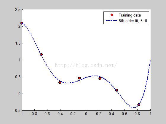
对输入特征参量x建模，通常x是个矢量，表示不同的特征。这里假设x是个标量，即只有一个特征，用5阶多项式拟合的预测函数：

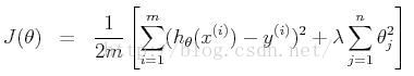
对输入样本数m大于多项式的阶数n，过拟合就很可能发生。为了避免这种情况，我们引入正规化因子λ。则代价函数：

对于线性回归，前面文章中提到了两种方法可解决，一种是梯度下降，二是公式法。

% Regularized linear regression
% Gradient descent
clc,clear,close all;
x = load('ex5Linx.dat');
y = load('ex5Liny.dat');

x_test = [-1: 0.01 : 1]';
x1 = [ones(size(x(:, 1)), 1), x, x.^2, x.^3, x.^4, x.^5];    % m * 6
x_test1 = [ones(size(x_test(:, 1)), 1), x_test, x_test.^2, x_test.^3, x_test.^4, x_test.^5];% test
[m, n] = size(x1);

theta = zeros(n, 1);
iter = 2000;
alpha = 0.07;
lamda = [0, 1, 10];         % regularized param
J_value = zeros(iter, 1);   % cost value
E = eye(n, n);
E(1, 1) = 0;
norm_gradient = zeros(length(lamda), 1);
for lamdaTemp = 1 : length(lamda)
    theta = zeros(n, 1);
    for iterTemp = 1 : iter
        h_theta = x1 * theta;  % m * 1
        J_value(iterTemp) = 1 / 2 / m * (sum((h_theta - y).^2)...
            + lamda(lamdaTemp) .* (sum(theta.^2) - theta(1).^2));
        theta = theta - alpha ./ m .* (x1' * (h_theta - y) + lamda(lamdaTemp) * E * theta); %iteration function
    end
    figure; scatter(x, y, 'o','LineWidth', 2, 'MarkerEdgeColor','k','MarkerFaceColor','r');
    hold on;
    plot(x_test, x_test1 * theta, '--b','LineWidth',2);
    legend(['Training data'],['5th order fit, λ=' num2str(lamda(lamdaTemp))]);
    figure; plot(1: iter, J_value);
    xlabel('iteration');
    ylabel('J_value');
    theta
    norm_gradient(lamdaTemp) = norm(theta);
end
norm_gradient

% Normal equations
norm_normal = zeros(length(lamda), 1);
for lamdaTemp = 1 : length(lamda)
    theta = pinv(x1' * x1 + lamda(lamdaTemp) .* E) * x1' * y
    norm_normal(lamdaTemp) = norm(theta);
    figure; scatter(x, y, 'o','LineWidth', 2, 'MarkerEdgeColor','k','MarkerFaceColor','r');
    hold on; plot(x_test, x_test1 * theta, '--b','LineWidth',2);
    legend(['Training data'],['5th order fit, λ=' num2str(lamda(lamdaTemp))]);
end
norm_normal

梯度下降法：

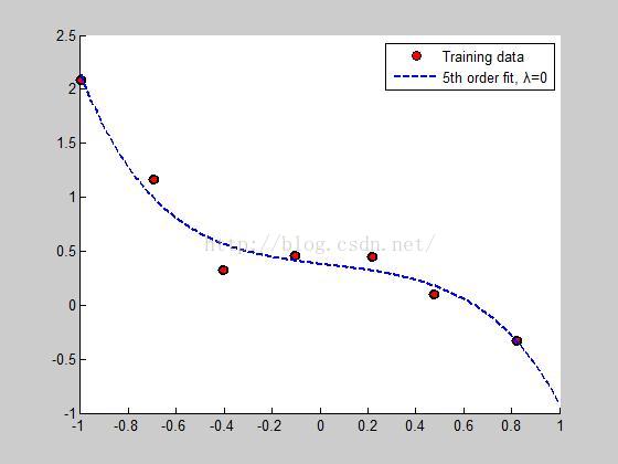
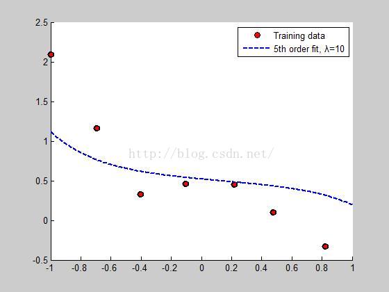
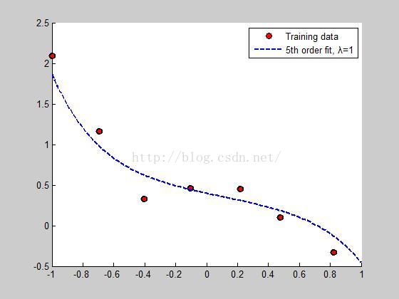
各自正规化因子对应的预测曲线如下：

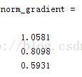
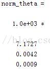
对应的范数：

公式法：

各自正规化因子对应的预测曲线如下：

对应的范数：

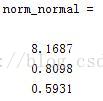
可以看出，随着λ 的增大，θ参量的范数下降。这是由于大的λ 补偿了原代价函数中大的参数。当λ 过大时，容易出现欠拟合，且预测曲线的走向与实际的相反。

logistic回归的正规化

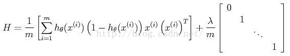
对于分类的logistic 回归，其正规化的代价函数：

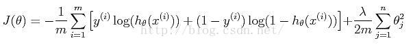
其中

，

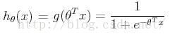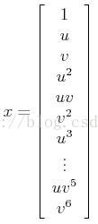
采用牛顿法求解最小代价函数。

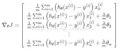
迭代函数：

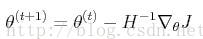
其中：

% Regularized Logistic regression
clear, clc, close all;
x = load('ex5Logx.dat');
y = load('ex5Logy.dat');

% Find the indices for the 2 classes
pos = find(y == 1); neg = find(y == 0);

g = inline('1.0 ./ (1.0 + exp(-z))');   % Usage: To find the value of the sigmoid 

degree = 6;
lamda = [0, 1, 10];
x1 = map_feature(x(:,1), x(:,2), degree);   % m * n
[m, n] = size(x1);
E = ones(n, 1);
E(1) = 0;
norm_lamda = zeros(length(lamda),1);

for lamdaTemp = 1 : length(lamda)
    theta = zeros(n, 1);
    J_theta = 0;
    thetaTemp = zeros(n, 1);
    J_thetaTemp = 0;
    while (1)
        h_theta = g(x1 * thetaTemp);       % m * 1
        J_thetaTemp = -1 ./ m * (sum(y .* log(h_theta) + (1 - y) .* log(1 - h_theta))...
            - lamda(lamdaTemp) ./ 2 * sum(thetaTemp.^2) - thetaTemp(1).^2)
        if (abs(J_theta - J_thetaTemp) < 0.0001)
            theta = thetaTemp
            break;
        end
        J_theta = J_thetaTemp;
        
        H = 1 ./ m * (x1' * diag(h_theta .*(1 - h_theta)) * x1 + lamda(lamdaTemp) .* diag(E));     % n * n
        delta_J = 1 ./ m * (x1' *  (h_theta - y) + lamda(lamdaTemp) .* diag(E) * thetaTemp);    % n * 1
        
        thetaTemp = thetaTemp - pinv(H) * delta_J;
    end
    norm_lamda(lamdaTemp) = norm(theta);
    
    figure;
    plot(x(pos, 1), x(pos, 2), '+', 'MarkerEdgeColor','k','MarkerFaceColor','k','MarkerSize',6);
    hold on;
    plot(x(neg, 1), x(neg, 2), 'o', 'MarkerEdgeColor','k','MarkerFaceColor','r','MarkerSize',6);
    
   %%
    % Define the ranges of the grid
    u = linspace(-1, 1.5, 200);
    v = linspace(-1, 1.5, 200);

    % Initialize space for the values to be plotted
    z = zeros(length(u), length(v));

    % Evaluate z = theta*x over the grid
    for i = 1:length(u)
        for j = 1:length(v)
            % Notice the order of j, i here!
            z(j,i) = map_feature(u(i), v(j))*theta;
        end
    end

    % Because of the way that contour plotting works
    % in Matlab, we need to transpose z, or
    % else the axis orientation will be flipped!
    %z = z';
    % Plot z = 0 by specifying the range [0, 0]
    hold on;
    contour(u,v,z, [0, 0], 'g', 'LineWidth', 2);
    xlabel('u');
    ylabel('v');
    legend('y = 1', 'y = 0', 'Decision boundary');
    title(['λ = ' num2str(lamda(lamdaTemp))]);
end

vpa(norm_lamda, 8);
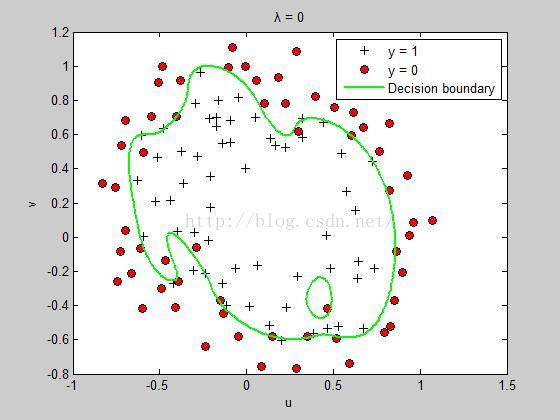
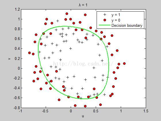
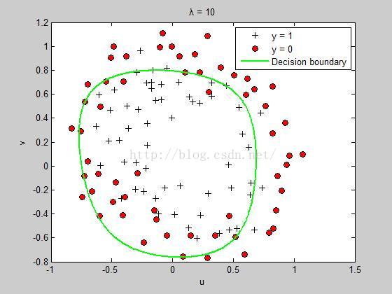
norm_lamda

各自正规化因子对应的预测曲线如下：

对应的范数：

当λ 增大时，θ 参量的范数减小。但是大到一定程度后也存在边界欠拟合的状况。