


- 🍨 本文为🔗365天深度学习训练营中的学习记录博客
- 🍖 原作者:K同学啊
我的环境:
● 语言环境:Python3.9
● 编译器:Jupyter lab
● 深度学习环境:
○ TensorFlow2.9.0+cuda11.2
○ 显卡:4060
一、前期准备
1.设置GPU
from tensorflow       import keras
from tensorflow.keras import layers,models
import os, PIL, pathlib
import matplotlib.pyplot as plt
import tensorflow        as tf

gpus = tf.config.list_physical_devices("GPU")

if gpus:
    gpu0 = gpus[0]                                        #如果有多个GPU,仅使用第0个GPU
    tf.config.experimental.set_memory_growth(gpu0, True)  #设置GPU显存用量按需使用
    tf.config.set_visible_devices([gpu0],"GPU")

gpus
2.导入查看数据
data_dir = "F:/DATA/DL/46-data"

data_dir = pathlib.Path(data_dir)

image_count = len(list(data_dir.glob('*/*/*.jpg')))
print("图片总数为:",image_count)

roses = list(data_dir.glob('train/nike/*.jpg'))
PIL.Image.open(str(roses[0]))
二、数据预处理
1.加载数据
batch_size = 32
img_height = 224
img_width = 224
"""
关于image_dataset_from_directory()的详细介绍可以参考文章:https://mtyjkh.blog.csdn.net/article/details/117018789
"""
train_ds = tf.keras.preprocessing.image_dataset_from_directory(
"F:/DATA/DL/46-data/train",
seed=123,
image_size=(img_height, img_width),
batch_size=batch_size)
"""
关于image_dataset_from_directory()的详细介绍可以参考文章:https://mtyjkh.blog.csdn.net/article/details/117018789
"""
val_ds = tf.keras.preprocessing.image_dataset_from_directory(
"F:/DATA/DL/46-data/test/",
seed=123,
image_size=(img_height, img_width),
batch_size=batch_size)
class_names = train_ds.class_names
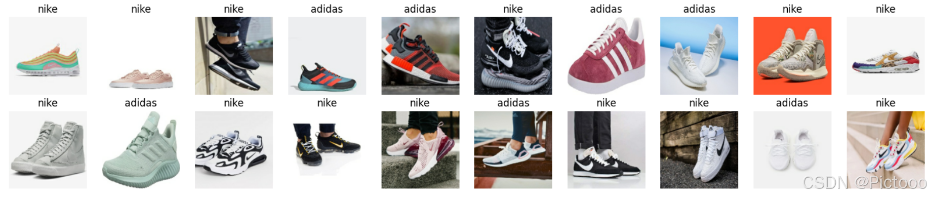
print(class_names)2.可视化
plt.figure(figsize=(20, 10))

for images, labels in train_ds.take(1):
    for i in range(20):
        ax = plt.subplot(5, 10, i + 1)

        plt.imshow(images[i].numpy().astype("uint8"))
        plt.title(class_names[labels[i]])

        plt.axis("off")

for image_batch, labels_batch in train_ds:
    print(image_batch.shape)
    print(labels_batch.shape)
    break

"""
● Image_batch是形状的张量(32,224,224,3)。这是一批形状224x224x3的32张图片(最后一维指的是彩色通道RGB)。
● Label_batch是形状(32,)的张量,这些标签对应32张图片
"""
3.配置数据
AUTOTUNE = tf.data.AUTOTUNE

train_ds = train_ds.cache().shuffle(1000).prefetch(buffer_size=AUTOTUNE)
val_ds = val_ds.cache().prefetch(buffer_size=AUTOTUNE)
三、构建CNN
"""
关于卷积核的计算不懂的可以参考文章:https://blog.csdn.net/qq_38251616/article/details/114278995

layers.Dropout(0.4) 作用是防止过拟合,提高模型的泛化能力。
关于Dropout层的更多介绍可以参考文章:https://mtyjkh.blog.csdn.net/article/details/115826689
"""

model = models.Sequential([
    layers.experimental.preprocessing.Rescaling(1./255, input_shape=(img_height, img_width, 3)),

    layers.Conv2D(16, (3, 3), activation='relu', input_shape=(img_height, img_width, 3)), # 卷积层1,卷积核3*3
    layers.AveragePooling2D((2, 2)),               # 池化层1,2*2采样
    layers.Conv2D(32, (3, 3), activation='relu'),  # 卷积层2,卷积核3*3
    layers.AveragePooling2D((2, 2)),               # 池化层2,2*2采样
    layers.Dropout(0.3),
    layers.Conv2D(64, (3, 3), activation='relu'),  # 卷积层3,卷积核3*3
    layers.Dropout(0.3),

    layers.Flatten(),                       # Flatten层,连接卷积层与全连接层
    layers.Dense(128, activation='relu'),   # 全连接层,特征进一步提取
    layers.Dense(len(class_names))               # 输出层,输出预期结果
])

model.summary() # 打印网络结构 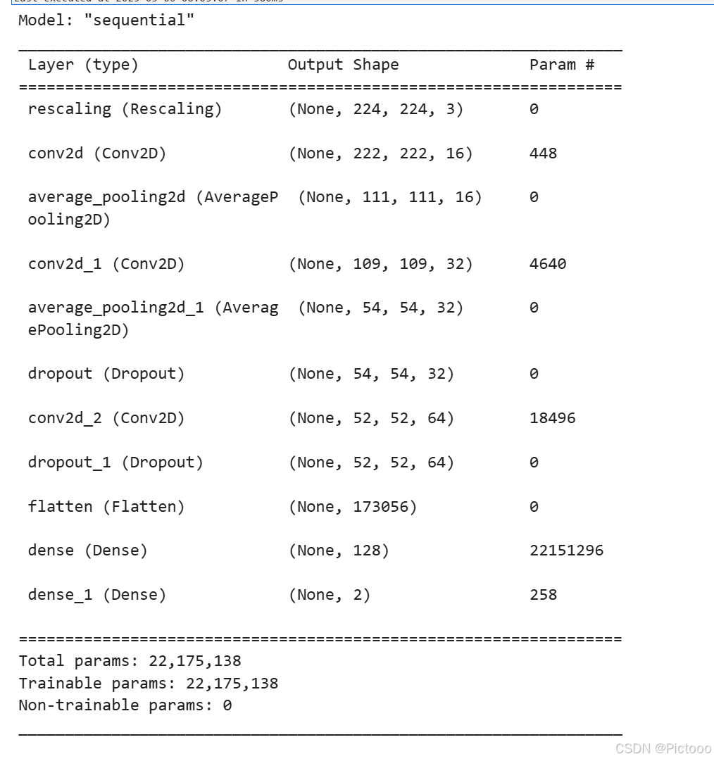
四、训练模型
# 设置初始学习率
initial_learning_rate = 0.001

lr_schedule = tf.keras.optimizers.schedules.ExponentialDecay(
        initial_learning_rate,
        decay_steps=10,      # 敲黑板!!!这里是指 steps,不是指epochs
        decay_rate=0.92,     # lr经过一次衰减就会变成 decay_rate*lr
        staircase=True)

# 将指数衰减学习率送入优化器
optimizer = tf.keras.optimizers.Adam(learning_rate=lr_schedule)

model.compile(optimizer=optimizer,
              loss=tf.keras.losses.SparseCategoricalCrossentropy(from_logits=True),
              metrics=['accuracy'])

from tensorflow.keras.callbacks import ModelCheckpoint, EarlyStopping

epochs = 50

# 保存最佳模型参数
checkpointer = ModelCheckpoint('best_model_T5.h5',
                                monitor='val_accuracy',
                                verbose=1,
                                save_best_only=True,
                                save_weights_only=True)

# 设置早停
earlystopper = EarlyStopping(monitor='val_accuracy',
                             min_delta=0.001,
                             patience=20,
                             verbose=1)

history = model.fit(train_ds,
                    validation_data=val_ds,
                    epochs=epochs,
                    callbacks=[checkpointer, earlystopper])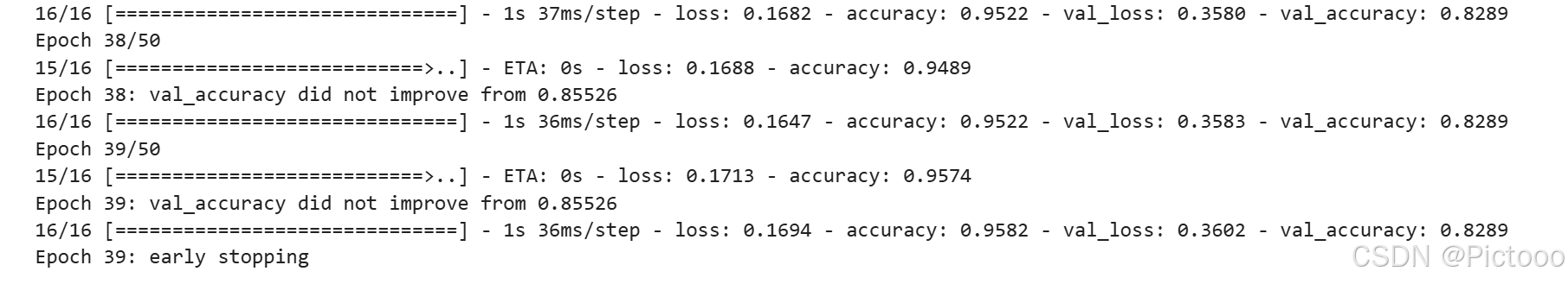
五、模型评估
from datetime import datetime
current_time = datetime.now() # 获取当前时间

acc = history.history['accuracy']
val_acc = history.history['val_accuracy']

loss = history.history['loss']
val_loss = history.history['val_loss']

epochs_range = range(len(loss))

plt.figure(figsize=(12, 4))
plt.subplot(1, 2, 1)
plt.plot(epochs_range, acc, label='Training Accuracy')
plt.plot(epochs_range, val_acc, label='Validation Accuracy')
plt.legend(loc='lower right')
plt.title('Training and Validation Accuracy')
plt.xlabel(current_time) # 打卡请带上时间戳,否则代码截图无效

plt.subplot(1, 2, 2)
plt.plot(epochs_range, loss, label='Training Loss')
plt.plot(epochs_range, val_loss, label='Validation Loss')
plt.legend(loc='upper right')
plt.title('Training and Validation Loss')
plt.show() 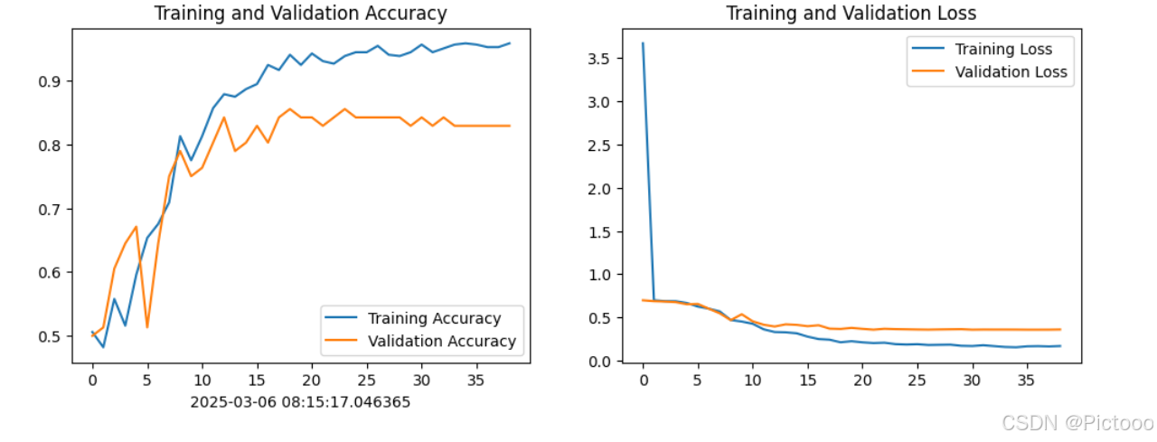
六、总结
学习率大与学习率小的优缺点分析:
学习率大
- 优点:
-
- 1、加快学习速率。
-
- 2、有助于跳出局部最优值。
- 缺点:
-
- 1、导致模型训练不收敛。
-
- 2、单单使用大学习率容易导致模型不精确。
学习率小
- 优点:
-
- 1、有助于模型收敛、模型细化。
-
- 2、提高模型精度。
- 缺点:
-
- 1、很难跳出局部最优值。
-
- 2、收敛缓慢。


 被折叠的 条评论
为什么被折叠?
被折叠的 条评论
为什么被折叠?
 到【灌水乐园】发言


