关于哪吒2票房的一份预测

对于现在火热的电影《哪吒2》的票房的未来我们十分好奇，并十分期待它最终能在全球票房排名上居于何位。那么如下就是关于它的一份具体预测以及过程：

一、时间序列预测

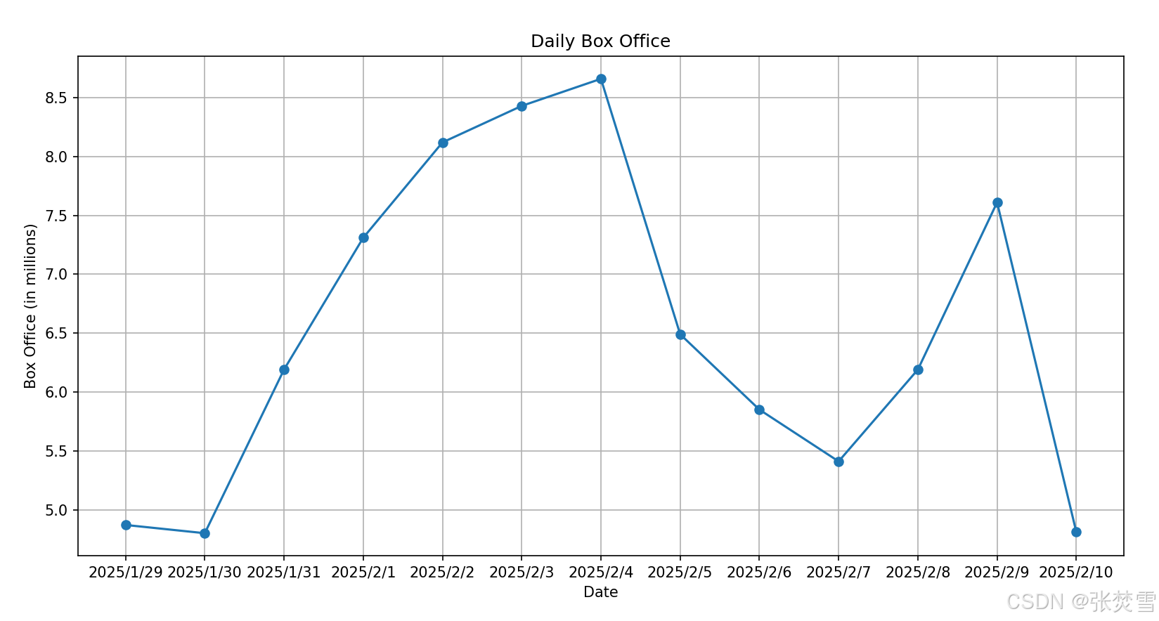
开始，我们考虑能否不引入多变量，而只靠过去几天的票房数据来进行时间序列预测，但我们需要先计算它的ADF统计量与p值，发现初始数据的ADF统计量与p值并不满足要求，所以进行差分，得到如下的结果： 

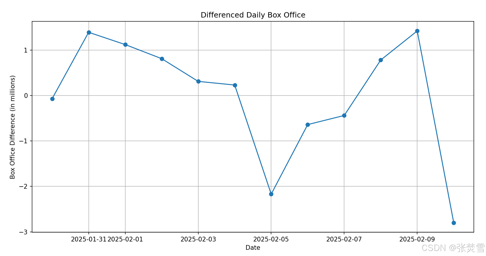
# 一次差分
ADF Statistic: -2.135221
p-value: 0.230590
# 二次差分
ADF Statistic: -2.207316
p-value: 0.203601

通过结果发现进行一阶差分与二阶差分后数据依然不够稳定，无法进行时间序列数据，所以放弃时间序列数据预测的策略，而考虑机器学习中的回归算法，比如线性回归、岭回归或Lasso回归。 

此外，为了直观感受数据的不平稳性，我还进行的绘图，图表如下：

二、回归算法

2.1 特征值处理

如果我们要用回归算法取预测未来数据，那么就需要更多的特征变量，因此通过“猫眼”中的票房数据进行补全，并考虑某日是否数据节假日。那么得到了特征变量如下：

['Date', 'Box_office', 'Holiday', 'Box_Percentage', 'Screening_schedule', 'Screening_percentage', 'Avg_people_showing', 'Occupancy_rate']

其中是否是假期的特征变量十分容易知道，只需要依靠日历即可，那么我们需要知道之后知道2月28日的其他所有变量的值。

首先看排片场次，我们考虑通过时间序列预测来预测未来的排片场次，并且通过计算ADF统计量和p值得到如下结果：

# Screening_schedule
The ADF Statistic: -2.972511550757476
The P-value: 0.037542443197409826

 然后画原始数据的折线图以及ADF统计量：

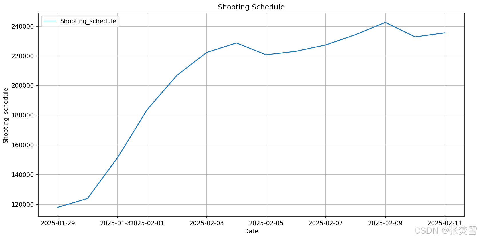
综上，数据明显是平稳的，因此可以考虑时间序列预测，那么通过ARIMA模型预测得到如下结果： 

# predict
2025-02-12    235474.580074
2025-02-13    235142.775054
2025-02-14    234894.423029
2025-02-15    234708.534555
2025-02-16    234569.399292
2025-02-17    234465.258238
2025-02-18    234387.309925
2025-02-19    234328.966559
2025-02-20    234285.297259
2025-02-21    234252.611319
2025-02-22    234228.146290
2025-02-23    234209.834513
2025-02-24    234196.128370
2025-02-25    234185.869489
2025-02-26    234178.190841
2025-02-27    234172.443466
2025-02-28    234168.141626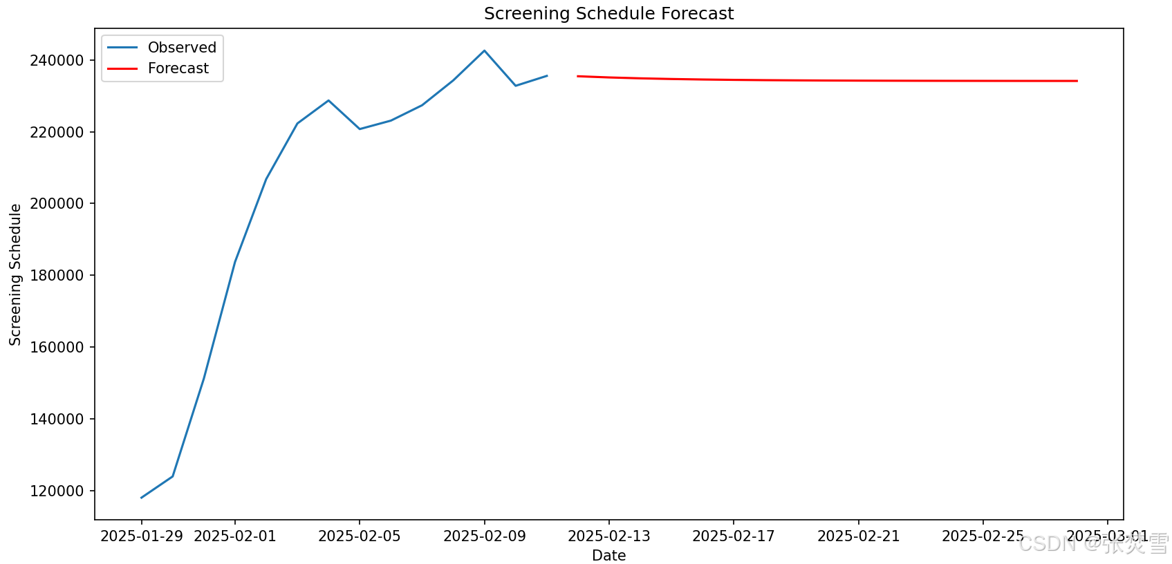

 然后是票房占比，我们采取同样的方法，得到了ADF统计量以及p值如下并画图得：

# Box_percentage
The ADF Statistic: -4.5369050230208225
The P-value: 0.00016855377365147394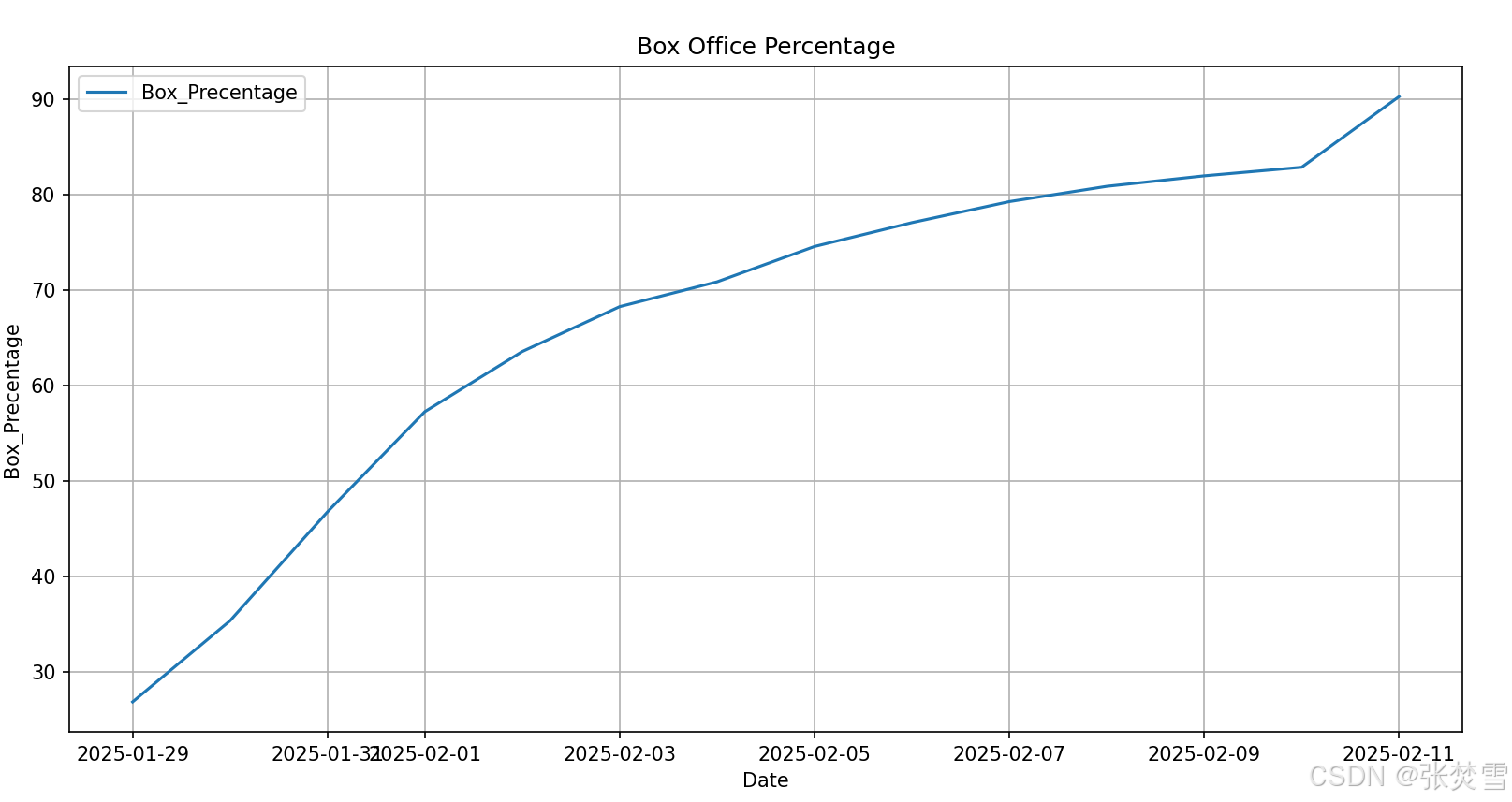

如果我们采取与刚才一样的方法，就会出现问题，因为这里这个特征值是一个百分比的数，持续增长就是超过100%，但这样与实际不符，并且考虑之后可能存在的一个下降趋势，所以我们这里简单采用将当前最后的一个票房占比值作为未来预测的第一个值，并每日递减1%，即从89%开始逐日地间1%。

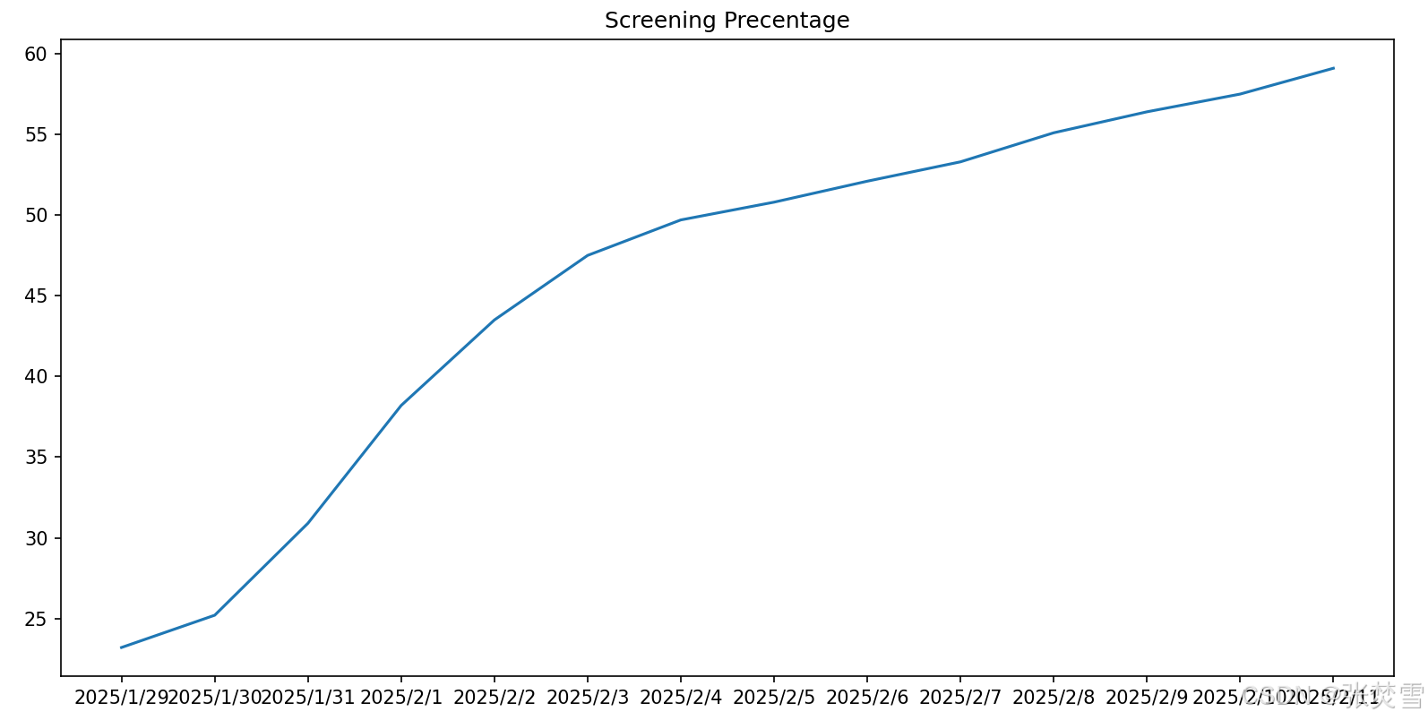
接着是排片场次，我们通过ADF统计量与p值发现该数据并不平稳，因此不能通过时间序列预测，然后通过画图（如下）发现它也是一个逐渐增加的趋势，但出于与票房占比一样的考虑，我们采取一样的方法，即从59.3%逐日递减1%。

接着是场均人次与上座率，ADF统计量与p值同样显示我们不能正常用时间序列预测，所以先画图：

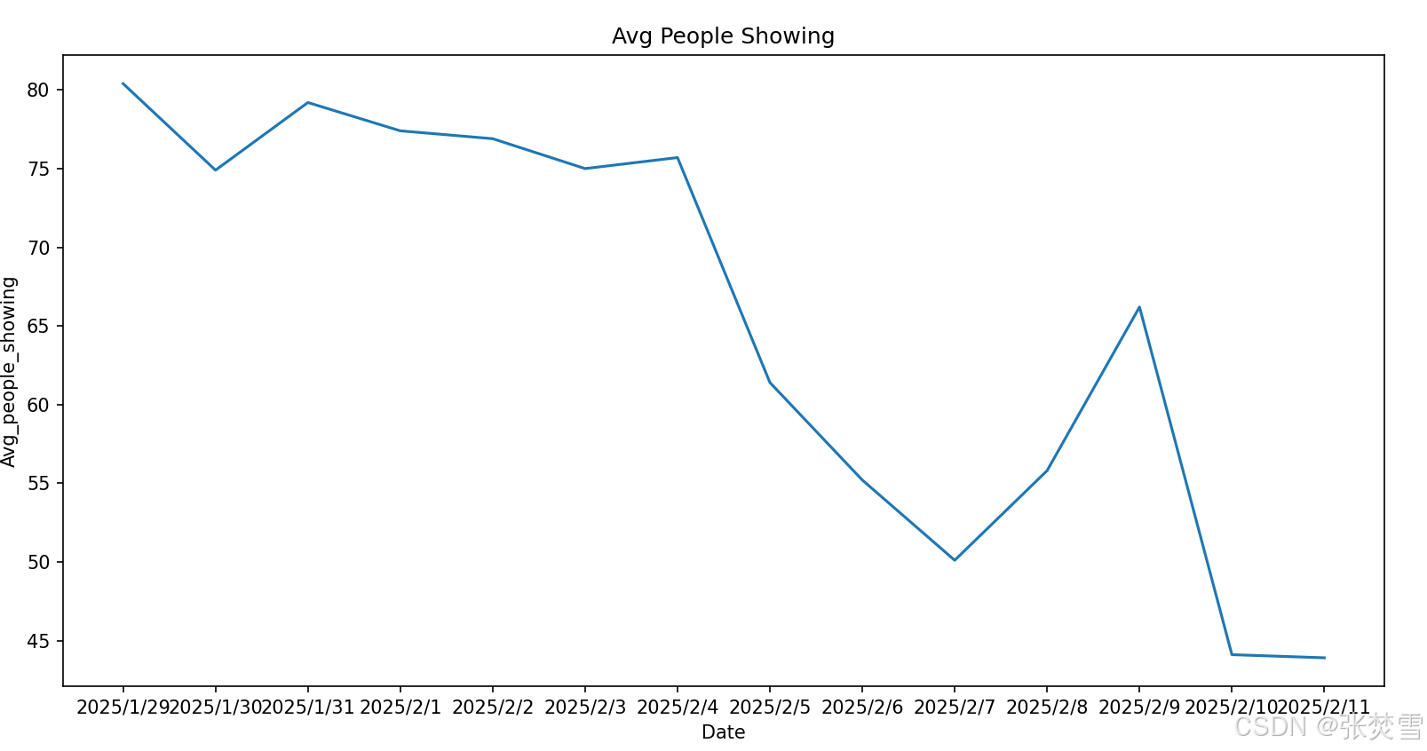
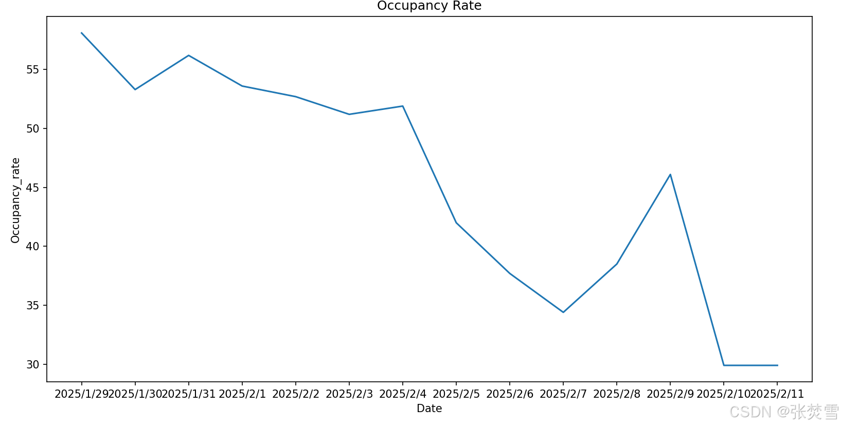
在这里，我们仅仅采用将已知的最后一日的数据作为之后的所有日的对应特征的值，即场均人次与上座率在之后将一直分别保持43.9与29.9。

2.2 线性回归预测

接下来进行预测，我们采用线性回归的技术。因为数据集较小，而线性回归十分适合于较小的数据集预测。

首先我们有两个数据集，一个是过去票房的数据集，一个是未来还没有票房数据只有其他特征值的数据集，并且对于两个数据集中的‘Date’特征值进行这样的处理，即将原本2025-2-12的值转化为Unix时间戳的形式——1707724800。然后进行ML中对应的操作即可，因此得到了代码如下：

import pandas as pd
import numpy as np
from sklearn.model_selection import train_test_split
from sklearn.linear_model import LinearRegression
from sklearn.metrics import mean_squared_error, r2_score
from sklearn.preprocessing import StandardScaler

# Load data
path = r"C:\Users\20349\Desktop\STUDING\COMPUTER\ArtificialIntelligence\data_set\box_office.csv"
box_office = pd.read_csv(path)
path_predict = r"C:\Users\20349\Desktop\STUDING\COMPUTER\ArtificialIntelligence\data_set\dataset\box_office_predict.csv"
box_office_predict = pd.read_csv(path_predict)

# Convert 'Date' to Unix timestamp and extract additional features
box_office['Date'] = pd.to_datetime(box_office['Date'])
box_office['Timestamp'] = (box_office['Date'] - pd.Timestamp("1970-01-01")) // pd.Timedelta('1s')

box_office_predict['Date'] = pd.to_datetime(box_office_predict['Date'])
box_office_predict['Timestamp'] = (box_office_predict['Date'] - pd.Timestamp("1970-01-01")) // pd.Timedelta('1s')

# Prepare datasets
y = box_office['Box_office']
X = box_office.drop(columns=['Box_office', 'Date'])
X_forecast = box_office_predict.drop(columns=['Date', 'Box_office'])

# Split the data
X_train, X_test, y_train, y_test = train_test_split(X, y, test_size=0.2, random_state=2025)

# Feature scaling
scaler = StandardScaler()
X_train_scaled = scaler.fit_transform(X_train)
X_test_scaled = scaler.transform(X_test)
X_forecast_scaled = scaler.transform(X_forecast)

# Train a linear regression model
model = LinearRegression()
model.fit(X_train_scaled, y_train)

# Predict on the test set
y_pred = model.predict(X_test_scaled)

y_forecast = model.predict(X_forecast_scaled)

# Evaluate the model
mse = mean_squared_error(y_test, y_pred)
r2 = r2_score(y_test, y_pred)

print(f"MSE: {mse:.2f}, R^2: {r2:.2f}")

其输出为：

MSE: 0.01, R^2: 0.98

通过均方误差（MSE）与决定系数（）的值可以知道模型的误差较小，而且模型可以解释98%的变异性，说明对于数据的拟合非常好。

2.3 预测结果

接下来是关于未来票房预测的输出，代码如下：

n = 0
for day in range(12,29):
    print(f"On 2025-2-{day}, the box office is: {abs(y_forecast[n]):.2f}")
    n += 1

total = sum(y_forecast)
print(f"The total forecast box office is:{total:.2f}")

total_before = sum(box_office['Box_office'].tolist())
print(f"The total box office is:{total+total_before:.2f}")

此时，得到了输出：

On 2025-2-12, the box office is: 4.89
On 2025-2-13, the box office is: 4.92
On 2025-2-14, the box office is: 4.99
On 2025-2-15, the box office is: 5.01
On 2025-2-16, the box office is: 2.82
On 2025-2-17, the box office is: 5.24
On 2025-2-18, the box office is: 5.32
On 2025-2-19, the box office is: 5.40
On 2025-2-20, the box office is: 5.49
On 2025-2-21, the box office is: 5.57
On 2025-2-22, the box office is: 5.59
On 2025-2-23, the box office is: 5.68
On 2025-2-24, the box office is: 5.83
On 2025-2-25, the box office is: 5.91
On 2025-2-26, the box office is: 6.00
On 2025-2-27, the box office is: 6.08
On 2025-2-28, the box office is: 6.17
The total forecast box office is:85.26
The total box office is:174.81

结果显示最后票房值在没有意外的情况下是174.81亿，这样的票房结果十分优秀，它说明最后《哪吒2》能在全球票房中排到第3位的好位置。但这是过于乐观的，因为我们在预测未来的票房的数据集中采用了较为乐观的特征值，而在实际情况中，这些特征值往往会有一个递减的趋势，我们并没有在对于未来的数据的特征值中很好把握这个趋势，所以可以考虑在最后的结果上增加一个折扣因子，这里采用和RL中折扣因子一样的表达方式，即gamma来表示。故得到代码如下：

gamma = 0.9
n = 0
for day in range(12,29):
    y_forecast[n] = abs(y_forecast[n])*gamma
    print(f"On 2025-2-{day}, the box office is: {y_forecast[n]:.2f}")
    n += 1

此处折扣因子大小的选择可以根据以往类似电影票房上的预测中折扣因子的选择，即我们采取同样的手段预测《哪吒1》、《大圣归来》、《神偷奶爸》等电影，并在在最后的预测上用网格搜索的方法，选择在乘以gamma后最逼近真实值的gamma值。（此处为了简便，先简单选择0.9）

这样，得到了输出：

On 2025-2-12, the box office is: 4.40
On 2025-2-13, the box office is: 4.43
On 2025-2-14, the box office is: 4.49
On 2025-2-15, the box office is: 4.51
On 2025-2-16, the box office is: 2.54
On 2025-2-17, the box office is: 4.71
On 2025-2-18, the box office is: 4.79
On 2025-2-19, the box office is: 4.86
On 2025-2-20, the box office is: 4.94
On 2025-2-21, the box office is: 5.01
On 2025-2-22, the box office is: 5.03
On 2025-2-23, the box office is: 5.11
On 2025-2-24, the box office is: 5.24
On 2025-2-25, the box office is: 5.32
On 2025-2-26, the box office is: 5.40
On 2025-2-27, the box office is: 5.47
On 2025-2-28, the box office is: 5.55
The total forecast box office is:81.82
The total box office is:171.37

虽然gamma能减少未来特征值估计中的误差，但实际存在的递减趋势还是没有很好的表达，所以，对于gamma进行改进，考虑让gamma逐日递减，以此来模拟实际票房中各个特征值中可能存在的递减趋势。那么修改后代码如下：

gamma = 0.95
n = 0
for day in range(12,29):
    y_forecast[n] = abs(y_forecast[n])*gamma
    print(f"On 2025-2-{day}, the box office is: {y_forecast[n]:.2f}")
    gamma -= 0.05
    n += 1

total = sum(y_forecast)
print(f"The total forecast box office is:{total:.2f}")

total_before = sum(box_office['Box_office'].tolist())
print(f"The total box office is:{total+total_before:.2f}")

此时得到了票房结果输出为：

On 2025-2-12, the box office is: 4.64
On 2025-2-13, the box office is: 4.43
On 2025-2-14, the box office is: 4.25
On 2025-2-15, the box office is: 4.01
On 2025-2-16, the box office is: 2.12
On 2025-2-17, the box office is: 3.66
On 2025-2-18, the box office is: 3.46
On 2025-2-19, the box office is: 3.24
On 2025-2-20, the box office is: 3.02
On 2025-2-21, the box office is: 2.79
On 2025-2-22, the box office is: 2.52
On 2025-2-23, the box office is: 2.27
On 2025-2-24, the box office is: 2.04
On 2025-2-25, the box office is: 1.77
On 2025-2-26, the box office is: 1.50
On 2025-2-27, the box office is: 1.22
On 2025-2-28, the box office is: 0.93
The total forecast box office is:47.85
The total box office is:137.40

在这样的一个思路下，gamma中间递减的幅度如何选择还是可以通过对于以往票房预测中的经验以及专家意见来选择。并且还可以为了增加一些不确定性而让gamma的递减是在一个合适的范围内随机选择来实现。

最后，在一个简单的估计中，最后《哪吒2》的票房结果是137.40亿，居于全球票房的第8位。

2.4 存在的问题

在上述的预测中，也许会存在一些其他的影响因素而使真实结果与预测结果存在较大的差异，这无法避免，但我们还可以利用集成学习等手段提高模型预测的精准性，比如再训练一个决策树、岭回归与Lasso回归与上述模型的预测结果取均值等手段来集成。

此外，还考虑gamma值以及每日减幅的选择的合适性，我这里没有用许多其他电影票房数据去寻找、检验最佳的gamma值以及减幅值，所以这里的误差也可能会有影响。

此上