


💥💥💞💞欢迎来到本博客❤️❤️💥💥
🏆博主优势:🌞🌞🌞博客内容尽量做到思维缜密,逻辑清晰,为了方便读者。
⛳️座右铭:行百里者,半于九十。
📋📋📋本文目录如下:🎁🎁🎁
目录
⛳️赠与读者
👨💻做科研,涉及到一个深在的思想系统,需要科研者逻辑缜密,踏实认真,但是不能只是努力,很多时候借力比努力更重要,然后还要有仰望星空的创新点和启发点。当哲学课上老师问你什么是科学,什么是电的时候,不要觉得这些问题搞笑。哲学是科学之母,哲学就是追究终极问题,寻找那些不言自明只有小孩子会问的但是你却回答不出来的问题。建议读者按目录次序逐一浏览,免得骤然跌入幽暗的迷宫找不到来时的路,它不足为你揭示全部问题的答案,但若能让人胸中升起一朵朵疑云,也未尝不会酿成晚霞斑斓的别一番景致,万一它居然给你带来了一场精神世界的苦雨,那就借机洗刷一下原来存放在那儿的“躺平”上的尘埃吧。
或许,雨过云收,神驰的天地更清朗.......🔎🔎🔎
💥1 概述
本文模拟了一个机器人在一个2D世界中巡航,世界中有5个独特可识别的地标,它们的位置未知。机器人配备了能够测量到这些地标距离和角度的传感器,但每个测量都受到噪声的影响。
这个实现基于Thrun等人的FastSLAM 1.0算法,算法通过粒子滤波器表示机器人的位置。每个粒子包含5个完全独立的扩展卡尔曼滤波器,每个滤波器负责跟踪一个地标。每次地标测量之后,根据最新地标测量与其预期的接近程度,给每个粒子评分。然后重新采样粒子,使得得分高的粒子可能会被复制,得分低的粒子可能会被删除。
2D 世界中的机器人巡航模拟
概述
本模拟文档描述了一个机器人在一个二维世界中巡航的过程。机器人在一个定义好的世界中移动,世界中有五个独特且可识别的地标,这些地标的位置对机器人来说是未知的。机器人配备了能够测量到这些地标的距离和角度的传感器,但每个测量都受到噪声的影响。此文档包括模拟环境的设定、传感器测量的实现及其结果的可视化。
世界设定
- **世界尺寸**:定义为100x100的二维空间。
- **地标**:五个独特的地标,位置未知但在模拟中预定义。
- **机器人初始位置**:在模拟开始时,机器人的位置在世界的中心,即坐标(50, 50)。
机器人和传感器
- **机器人位置**:机器人在二维空间中的当前坐标。
- **传感器噪声**:测量过程中加入的高斯噪声,标准差设定为1.0。角度测量噪声为距离噪声的10%。
代码实现
```python
import numpy as np
import matplotlib.pyplot as plt

# 设定世界参数
world_size = 100  # 世界的大小为100x100
landmarks = np.array([[20, 30], [80, 80], [50, 10], [20, 80], [80, 20]])  # 地标的位置

# 设定机器人参数
robot_pos = np.array([50, 50])  # 机器人的初始位置
sensor_noise_std = 1.0  # 传感器噪声的标准差

def sense(robot_pos, landmarks, sensor_noise_std):
    """模拟机器人传感器对地标的测量"""
    measurements = []
    for landmark in landmarks:
        distance = np.linalg.norm(landmark - robot_pos)
        angle = np.arctan2(landmark[1] - robot_pos[1], landmark[0] - robot_pos[0])

        # 加入噪声
        distance += np.random.normal(0, sensor_noise_std)
        angle += np.random.normal(0, sensor_noise_std * 0.1)

        measurements.append((distance, angle))
    return measurements

# 进行一次传感器测量
measurements = sense(robot_pos, landmarks, sensor_noise_std)

# 打印测量结果
print("测量结果(距离, 角度):")
for i, measurement in enumerate(measurements):
    print(f"地标 {i+1}: {measurement}")

# 可视化世界、地标和机器人的位置
plt.figure(figsize=(8, 8))
plt.xlim(0, world_size)
plt.ylim(0, world_size)
plt.scatter(landmarks[:, 0], landmarks[:, 1], color='red', label='Landmarks')
plt.scatter(robot_pos[0], robot_pos[1], color='blue', label='Robot')

# 画出测量线
for i, (distance, angle) in enumerate(measurements):
    lx, ly = robot_pos[0] + distance * np.cos(angle), robot_pos[1] + distance * np.sin(angle)
    plt.plot([robot_pos[0], lx], [robot_pos[1], ly], label=f'Measurement {i+1}')

plt.legend()
plt.grid()
plt.show()
主要步骤
1. **设定世界参数**:定义二维世界的尺寸和地标的位置。
2. **设定机器人参数**:定义机器人的初始位置和传感器的噪声水平。
3. **传感器测量**:通过 `sense` 函数模拟机器人对地标的测量,加入噪声。
4. **测量结果输出**:打印出每个地标的测量结果(包括距离和角度)。
5. **结果可视化**:使用 `matplotlib` 可视化世界、地标和机器人的位置,以及测量的结果。
扩展
可以根据需要进一步扩展这个模拟,例如:
- 添加机器人运动模型,模拟机器人在二维世界中的移动。
- 引入更多类型的噪声(如系统噪声)。
- 改变测量频率,以模拟不同传感器刷新率。
通过这些扩展,可以更加真实地模拟机器人在未知环境中的导航和定位过程。
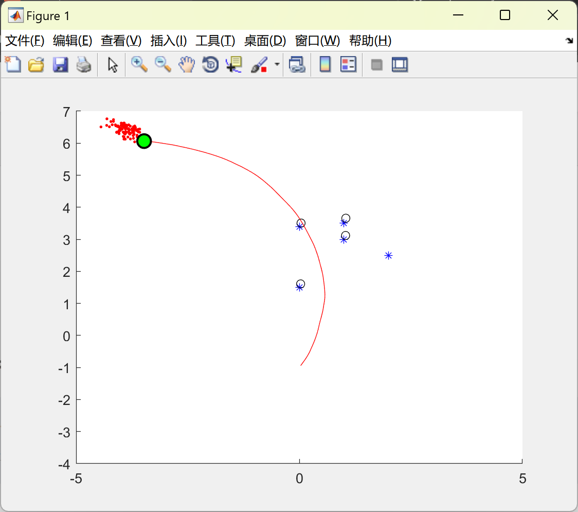
📚2 运行结果

部分代码:
% The number of timesteps for the simulation
timesteps = 200;
% The maximum distance from which our sensor can sense a landmark
max_read_distance = 1.5;
% The actual positions of the landmarks (each column is a separate landmark)
real_landmarks = [1.0, 2.0, 0.0, 0.0, 1.0; % x
3.0, 2.5 3.4, 1.5, 3.5; % y
0.0, 0.0 0.0, 0.0, 0.0]; % Nothing
% The initial starting position of the robot
real_position = [0.0; % x
-1.0; % y
pi/3.0]; % rotation
% The movement command given tot he robot at each timestep
movement_command = [.05; % Distance
.01]; % Rotation
% The Gaussian variance of the movement commands
movement_variance = [.1; % Distance
.05]; % Rotation
M = [movement_variance(1), 0.0;
0.0, movement_variance(2)];
% The Gaussian variance of our sensor readings
measurement_variance = [0.1; % Distance
0.01; % Angle
.0001]; % Landmark Identity
R = [measurement_variance(1), 0.0, 0.0;
0.0, measurement_variance(2), 0.0;
0.0, 0.0, measurement_variance(3)];
% Create the particles and initialize them all to be in the same initial
% position.
particles = [];
num_particles = 100;
for i = 1:num_particles
particles(i).w = 1.0/num_particles;
particles(i).position = real_position;
for lIdx=1:size(real_landmarks,2)
particles(i).landmarks(lIdx).seen = false;
end
end
pos_history = [];
%%%%%%%%%%%%%%%%%%%%%%%%%%%%%%%%%%%%%%%%%%%%%%%%%%%%%%%%%%%%%%%%%%%%%%
%%%%%%%%%%%%%%%%%%%%%%%%%%%%%%%%%%%%%%%%%%%%%%%%%%%%%%%%%%%%%%%%%%%%%%
% SIMULATION
%%%%%%%%%%%%%%%%%%%%%%%%%%%%%%%%%%%%%%%%%%%%%%%%%%%%%%%%%%%%%%%%%%%%%%
%%%%%%%%%%%%%%%%%%%%%%%%%%%%%%%%%%%%%%%%%%%%%%%%%%%%%%%%%%%%%%%%%%%%%%
for timestep = 1:timesteps
%%%%%%%%%%%%%%%%%%%%%%%%%%%%%%%%%%%%%%%%
% Move the actual robot
real_position = moveParticle(real_position, movement_command, movement_variance);
pos_history = [pos_history, real_position];
% Move the actual particles
for pIdx = 1:num_particles
particles(pIdx).position = moveParticle( ...
particles(pIdx).position, movement_command, movement_variance);
particles(pIdx).position(3) = real_position(3);
end
%%%%%%%%%%%%%%%%%%%%%%%%%%%%%%%%%%%%%%%%
% Try to take a reading from each landmark
doResample = false;
for lIdx = 1:size(real_landmarks,2)
real_landmark = real_landmarks(:, lIdx);
% Take a real (noisy) measurement from the robot to the landmark
[z_real, G] = getMeasurement(real_position, real_landmark, measurement_variance);
read_distance(lIdx) = z_real(1);
read_angle(lIdx) = z_real(2);
% If the landmark is close enough, then we can spot it
if(read_distance(lIdx) < max_read_distance)
doResample = true;
for pIdx = 1:num_particles
if(particles(pIdx).landmarks(lIdx).seen == false)
% If we have never seen this landmark, then we need to initialize it.
% We'll just use whatever first reading we recieved.
particles(pIdx).landmarks(lIdx).pos = [particles(pIdx).position(1) + cos(read_angle(lIdx))*read_distance(lIdx);
particles(pIdx).position(2) + sin(read_angle(lIdx))*read_distance(lIdx);
0];
% Initialize the landmark position covariance
particles(pIdx).landmarks(lIdx).E = inv(G) * R * inv(G)';
particles(pIdx).landmarks(lIdx).seen = true;
else
% Get an ideal reading to our believed landmark position (note 0 variance here).
[z_p, Gp] = getMeasurement(particles(pIdx).position, particles(pIdx).landmarks(lIdx).pos, [0;0]);
residual = z_real - z_p;
%Calculate the Kalman gain
Q = G' * particles(pIdx).landmarks(lIdx).E * G + R;
K = particles(pIdx).landmarks(lIdx).E * G * inv(Q);
% Mix the ideal reading, and our actual reading using the Kalman gain, and use the result
% to predict a new landmark position
particles(pIdx).landmarks(lIdx).pos = particles(pIdx).landmarks(lIdx).pos + K*(residual);
% Update the covariance of this landmark
particles(pIdx).landmarks(lIdx).E = (eye(size(K)) - K*G')*particles(pIdx).landmarks(lIdx).E;
% Update the weight of the particle
particles(pIdx).w = particles(pIdx).w * norm(2*pi*Q).^(-1/2)*exp(-1/2*(residual)'*inv(Q)*(residual));
end %else
end %pIdx
end %distance
end %for landmark
% Resample all particles based on their weights
if(doResample)
particles = resample(particles);
end
%%%%%%%%%%%%%%%%%%%%%%%%%%%%%%%%%%%%%%%%
%%%%%%%%%%%%%%%%%%%%%%%%%%%%%%%%%%%%%%%%
% PLOTTING
%%%%%%%%%%%%%%%%%%%%%%%%%%%%%%%%%%%%%%%%
%%%%%%%%%%%%%%%%%%%%%%%%%%%%%%%%%%%%%%%%
clf;
hold on;
% Plot the landmarks
for lIdx=1:size(real_landmarks,2)
plot(real_landmarks(1,lIdx), real_landmarks(2,lIdx), 'b*');
end
for lIdx = 1:size(real_landmarks,2)
if(particles(1).landmarks(lIdx).seen)
avg_landmark_guess =[0;0;0];
for pIdx = 1:length(particles)
avg_landmark_guess = avg_landmark_guess + particles(pIdx).landmarks(lIdx).pos;
end
avg_landmark_guess = avg_landmark_guess / length(particles);
plot(avg_landmark_guess(1), avg_landmark_guess(2), 'ko');
end
end
% Plot the particles
particles_pos = [particles.position];
plot(particles_pos(1,:), particles_pos(2,:), 'r.');
% Plot the real robot
plot(pos_history(1,:), pos_history(2,:), 'r');
w = .1;
l = .3;
x = real_position(1);
y = real_position(2);
t = real_position(3);
plot(real_position(1), real_position(2), 'mo', ...
'LineWidth',1.5, ...
'MarkerEdgeColor','k', ...
'MarkerFaceColor',[0 1 0], ...
'MarkerSize',10);
% Show the sensor measurement as an arrow
for lIdx=1:size(real_landmarks,2)
real_landmark = real_landmarks(:, lIdx);
if(read_distance(lIdx) < max_read_distance)
line([real_position(1), real_position(1)+cos(read_angle(lIdx))*read_distance(lIdx)], ...
[real_position(2), real_position(2)+sin(read_angle(lIdx))*read_distance(lIdx)]);
end
end
🎉3 参考文献
文章中一些内容引自网络,会注明出处或引用为参考文献,难免有未尽之处,如有不妥,请随时联系删除。
[1]李秀芳.面向水下机器人的水下目标检测算法研究[D].中国海洋大学[2024-06-25].
[2]王海涛.水下机器人自主导航算法的研究[D].中国海洋大学[2024-06-25].DOI:CNKI:CDMD:2.1014.367966.
🌈4 Matlab代码实现
资料获取,更多粉丝福利,MATLAB|Simulink|Python资源获取


 229
229

 被折叠的 条评论
为什么被折叠?
被折叠的 条评论
为什么被折叠?
 到【灌水乐园】发言


