机器学习：SVM算法（Python）

一、核函数

kernel_func.py

import numpy as np


def linear():
    """
    线性核函数
    :return:
    """
    def _linear(x_i, x_j):
        return np.dot(x_i, x_j)

    return _linear


def poly(degree=3, coef0=1.0):
    """
    多项式核函数
    :param degree: 阶次
    :param coef: 常数项
    :return:
    """
    def _poly(x_i, x_j):
        return np.power(np.dot(x_i, x_j) + coef0, degree)

    return _poly


def rbf(gamma=1.0):
    """
    高斯核函数
    :param gamma: 超参数
    :return:
    """
    def _rbf(x_i, x_j):
        x_i, x_j = np.asarray(x_i), np.asarray(x_j)
        if x_i.ndim <= 1:
            return np.exp(-np.dot(x_i - x_j, x_i - x_j) / (2 * gamma ** 2))
        else:
            return np.exp(-np.multiply(x_i - x_j, x_i - x_j).sum(axis=1) / (2 * gamma ** 2))
    return _rbf

二、SVM算法的实现

svm_smo_classifier.py

import copy
import random

import matplotlib.pyplot as plt

import kernel_func
import numpy as np


class SVMClassifier:
    """
    支持向量机二分类算法：硬间隔、软间隔、核函数，可做线性可分、非线性可分。SMO算法
    1. 训练样本的目标值限定编码为{0， 1}. SVM在fit时把0类别重编码为-1
    """

    def __init__(self, C=1.0, gamma=1.0, degree=3, coef0=1.0, kernel=None, kkt_tol=1e-3, alpha_tol=1e-3,
                 max_epochs=100):
        self.C = C  # 软间隔硬间隔的参数，硬间隔：适当增大C的值，软间隔：减少C值，允许部分样本不满足约束条件
        # self.gamma = gamma  # 径向基函数/高斯核函数超参数
        # self.degree = degree  # 多项式核函数的阶次
        # self.coef0 = coef0  # 多项式核函数的常数项
        self.kernel = kernel  # 选择的核函数
        if self.kernel is None or self.kernel.lower() == "linear":
            self.kernel_func = kernel_func.linear()  # self.kernel_func(x_i, x_j)
        elif self.kernel.lower() == "poly":
            self.kernel_func = kernel_func.poly(degree, coef0)  # self.kernel_func(x_i, x_j)
        elif self.kernel.lower() == "rbf":
            self.kernel_func = kernel_func.rbf(gamma)
        else:
            print("仅限linear、poly或rbf，值为None则默认为Linear线性核函数...")
            self.kernel_func = kernel_func.linear()

        self.alpha_tol = alpha_tol  # 支持向量容忍度

        self.kkt_tol = kkt_tol  # 在精度内检查
        self.max_epochs = max_epochs
        self.alpha = None  # 松弛变量
        self.E = None  # 误差
        self.w, self.b = None, None  # SVM的模型系数

        self.support_vectors = []  # 记录支持向量的索引
        self.support_vectors_alpha = []  # 支持向量所对应的松弛变量
        self.support_vectors_x, self.support_vectors_y = [], []  # 支持向量所对应的样本和目标
        self.cross_entropy_loss = []  # 优化过程中的交叉熵损失

    def init_params(self, x_train, y_train):
        """
        初始化必要参数
        :param x_train: 训练集
        :param y_train: 编码后的目标集
        :return:
        """
        n_samples, n_features = x_train.shape
        self.w, self.b = np.zeros(n_features), 0.0  # 模型系数初始化为0值
        self.alpha = np.zeros(n_samples)  # 松弛变量
        self.E = self.decision_func(x_train) - y_train  # 初始化误差，所有样本类别取反

    def decision_func(self, x):
        """
        SVM模型的预测计算，
        :param x: 可以是样本集，也可以是单个样本
        :return:
        """
        if len(self.support_vectors) == 0:  # 当前没有支持向量
            if x.ndim <= 1:  # 标量或单个样本
                return 0
            else:
                return np.zeros(x.shape[0])  # np.zeros(x.shape[:-1])
        else:
            if x.ndim <= 1:
                wt_x = 0.0  # 模型w^T * x + b的第一项求和
            else:
                wt_x = np.zeros(x.shape[0])
            for i in range(len(self.support_vectors)):
                # 公式：w^T * x = sum(alpha_i * y_i * k(xi, x))
                wt_x += self.support_vectors_alpha[i] * self.support_vectors_y[i] * \
                        self.kernel_func(x, self.support_vectors_x[i])
        return wt_x + self.b

    def _meet_kkt(self, x_i, y_i, alpha_i, sample_weight_i):
        """
        判断当前需要优化的alpha是否满足KKT条件
        :param x_i: 已选择的样本
        :param y_i: 已选择的目标
        :param alpha_i: 需要优化的alpha
        :return: bool：满足True，不满足False
        """
        if alpha_i < self.C * sample_weight_i:
            return y_i * self.decision_func(x_i) >= 1 - self.kkt_tol
        else:
            return y_i * self.decision_func(x_i) <= 1 + self.kkt_tol

    def _select_best_j(self, best_i):
        """
        基于已经选择的第一个alpha_i，寻找使得|E_i - E_j|最大的best_j
        :param best_i: 已选择的第一个alpha_i索引
        :return:
        """
        valid_j_list = [j for j in range(len(self.alpha)) if self.alpha[j] > 0 and best_i != j]
        if len(valid_j_list) > 0:
            idx = np.argmax(np.abs(self.E[best_i] - self.E[valid_j_list]))  # 在可选的j列表中查找绝对误差最大的索引
            best_j = valid_j_list[int(idx)]  # 最佳的j
        else:
            idx = list(range(len(self.alpha)))  # 所有样本索引
            seq = idx[:best_i] + idx[best_i + 1:]  # 排除best_i
            best_j = random.choice(seq)  # 随机选择
        return best_j

    def _clip_alpha_j(self, y_i, y_j, alpha_j_unc, alpha_i_old, alpha_j_old, sample_weight_j):
        """
        修剪第2个更新的alpha值
        :param y_i: 当前选择的第1个y目标值
        :param y_j: 当前选择的第2个y目标值
        :param alpha_j_unc: 当前未修剪的第2个alpha值
        :param alpha_i_old: 当前选择的第1个未更新前的alpha值
        :param alpha_j_old: 当前选择的第2个未更新前的alpha值
        :return:
        """
        C = self.C * sample_weight_j
        if y_i == y_j:
            inf = max(0, alpha_i_old + alpha_j_old - C)  # L
            sup = min(self.C, alpha_i_old + alpha_j_old)  # H
        else:
            inf = max(0, alpha_j_old - alpha_i_old)  # L
            sup = min(C, C + alpha_j_old - alpha_i_old)  # H
        # if alpha_j_unc < inf:
        #     alpha_j_new = inf
        # elif alpha_j_unc > sup:
        #     alpha_j_new = sup
        # else:
        #     alpha_j_new = alpha_j_unc
        alpha_j_new = [inf if alpha_j_unc < inf else sup if alpha_j_unc > sup else alpha_j_unc]
        return alpha_j_new[0]

    def _update_error(self, x_train, y_train, y):
        """
        更新误差，计算交叉熵损失
        :param x_train: 训练样本集
        :param y_train: 目标集
        :param y: 编码后的目标集
        :return:
        """
        y_predict = self.decision_func(x_train)  # 当前优化过程中的模型预测值
        self.E = y_predict - y  # 误差
        loss = -(y_train.T.dot(np.log(self.sigmoid(y_predict))) +
                 (1 - y_train).T.dot(np.log(1 - self.sigmoid(y_predict))))
        self.cross_entropy_loss.append(loss / len(y))  # 平均交叉熵损失

    def fit(self, x_train, y_train, samples_weight=None):
        """
        SVM的训练：SMO算法实现
        1. 按照启发式方法选择一对需要优化的alpha
        2. 对参数alpha、b、w、E等进行更新、修剪
        :param x_train: 训练集
        :param y_train: 目标集
        :return:
        """
        x_train, y_train = np.asarray(x_train), np.asarray(y_train)
        if samples_weight is None:
            samples_weight = np.array([1.0] * x_train.shape[0])
        class_values = np.sort(np.unique(y_train))  # 类别的不同取值
        if class_values[0] != 0 or class_values[1] != 1:
            raise ValueError("仅限二分类，类别编码为{0、1}...")
        y = copy.deepcopy(y_train)
        y[y == 0] = -1  # SVM类别限定为{-1， 1}
        self.init_params(x_train, y)  # 参数的初始化
        n_samples = x_train.shape[0]  # 样本量
        for epoch in range(self.max_epochs):
            if_all_match_kkt_condition = True  # 表示所有样本都满足KKT条件
            # 1. 选择一对需要优化的alpha_i和alpha_j
            for i in range(n_samples):  # 外层循环
                x_i, y_i = x_train[i, :], y[i]  # 当前选择的第1个需要优化的样本所对应的索引
                alpha_i_old, err_i_old = self.alpha[i], self.E[i]  # 取当前未更新的alpha和误差
                if not self._meet_kkt(x_i, y_i,alpha_i_old, samples_weight[i]):  # 不满足KKT条件
                    if_all_match_kkt_condition = False  # 表示存在需要优化的变量
                    j = self._select_best_j(i)  # 基于alpha_i选择alpha_j
                    alpha_j_old, err_j_old = self.alpha[j], self.E[j]  # 当前第2个需要优化的alpha和误差
                    x_j, y_j = x_train[j, :], y[j]  # 第2个需要优化的样本所对应的索引

                    # 2. 基于已经选择的alpha_i和alpha_j，对alpha、b、E和w进行更新
                    # 首先获取未修建的第2个需要更新的alpha值，并对其进行修建
                    k_ii = self.kernel_func(x_i, x_i)
                    k_jj = self.kernel_func(x_j, x_j)
                    k_ij = self.kernel_func(x_i, x_j)
                    eta = k_ii + k_jj - 2 * k_ij
                    if np.abs(eta) < 1e-3:  # 避免分母过小，表示选择更新的两个样本比较接近
                        continue
                    alpha_j_unc = alpha_j_old - y_j * (err_j_old - err_i_old) / eta  # 未修剪的alpha_j
                    # 修剪alpha_j使得0< alpha_j < C
                    alpha_j_new = self._clip_alpha_j(y_i, y_j, alpha_j_unc, alpha_i_old,
                                                     alpha_j_old, samples_weight[j])

                    # 3. 通过修剪后的alpha_j_new更新alpha_i
                    alpha_j_delta = alpha_j_new - alpha_j_old
                    alpha_i_new = alpha_i_old - y_i * y_j * alpha_j_delta
                    self.alpha[i], self.alpha[j] = alpha_i_new, alpha_j_new  # 更新回存

                    # 4. 更新模型系数w和b
                    alpha_i_delta = alpha_i_new - alpha_i_old
                    # w的更新仅与已更新的一对alpha有关
                    self.w = self.w + alpha_i_delta * y_i * x_i + alpha_j_delta * y_j * x_j
                    b_i_delta = -self.E[i] - y_i * k_ii * alpha_i_delta - y_i * k_ij * alpha_j_delta
                    b_j_delta = -self.E[j] - y_i * k_ij * alpha_i_delta - y_i * k_jj * alpha_j_delta
                    if 0 < alpha_i_new < self.C * samples_weight[i]:
                        self.b += b_i_delta
                    elif 0 < alpha_j_new < self.C * samples_weight[j]:
                        self.b += b_j_delta
                    else:
                        self.b += (b_i_delta + b_j_delta) / 2

                    # 5. 更新误差E，计算损失
                    self._update_error(x_train, y_train, y)

                    # 6. 更新支持向量相关信息，即重新选取
                    self.support_vectors = np.where(self.alpha > self.alpha_tol)[0]
                    self.support_vectors_x = x_train[self.support_vectors, :]
                    self.support_vectors_y = y[self.support_vectors]
                    self.support_vectors_alpha = self.alpha[self.support_vectors]
            if if_all_match_kkt_condition:  # 没有需要优化的alpha，则提前停机
                break

    def get_params(self):
        """
        获取SVM的模型系数
        :return:
        """
        return self.w, self.b

    def predict_proba(self, x_test):
        """
        预测测试样本所属类别的概率
        :param x_test: 测试样本集
        :return:
        """
        x_test = np.asarray(x_test)
        y_test_hat = np.zeros((x_test.shape[0], 2))  # 存储每个样本的预测概率
        y_test_hat[:, 1] = self.sigmoid(self.decision_func(x_test))
        y_test_hat[:, 0] = 1.0 - y_test_hat[:, 1]
        return y_test_hat

    def predict(self, x_test):
        """
        预测测试样本的所属类别
        :param x_test: 测试样本集
        :return:
        """
        return np.argmax(self.predict_proba(x_test), axis=1)

    @staticmethod
    def sigmoid(x):
        """
        sigmodi函数，为避免上溢或下溢，对参数x做限制
        :param x: 可能是标量数据，也可能是数组
        :return:
        """
        x = np.asarray(x)  # 为避免标量值的布尔索引出错，转换为数组
        x[x > 30.0] = 30.0  # 避免下溢
        x[x < -50.0] = -50.0  # 避免上溢
        return 1 / (1 + np.exp(-x))

    def plt_loss_curve(self, is_show=True):
        """
        可视化交叉熵损失函数
        :param is_show:
        :return:
        """
        if is_show:
            plt.figure(figsize=(7, 5))
        plt.plot(self.cross_entropy_loss, "k-", lw=1)
        plt.xlabel("Training Epochs", fontdict={"fontsize": 12})
        plt.ylabel("The Mean of Cross Entropy Loss", fontdict={"fontsize": 12})
        plt.title("The SVM Loss Curve of Cross Entropy")
        plt.grid(ls=":")
        if is_show:
            plt.show()

    def plt_svm(self, X, y, is_show=True, is_margin=False):
        """
        可视化支持向量机模型：分类边界、样本、间隔、支持向量
        :param X:
        :param y:
        :param is_show:
        :return:
        """
        X, y = np.asarray(X), np.asarray(y)
        if is_show:
            plt.figure(figsize=(7, 5))
        if X.shape[1] != 2:
            print("Warning: 仅限于两个特征的可视化...")
            return

        # 可视化分类填充区域
        x_min, x_max = X[:, 0].min() - 1, X[:, 0].max() + 1
        y_min, y_max = X[:, 1].min() - 1, X[:, 1].max() + 1
        xi, yi = np.meshgrid(np.linspace(x_min, x_max, 100), np.linspace(y_min, y_max, 100))
        zi = self.predict(np.c_[xi.ravel(), yi.ravel()])
        zi = zi.reshape(xi.shape)  # 等值线的x、y和z的维度必须一致
        plt.contourf(xi, yi, zi, cmap="winter", alpha=0.3)

        # 可视化正例、负例样本
        positive, negative = X[y == 1.0], X[y == 0.0]
        plt.plot(positive[:, 0], positive[:, 1], "*", label="Positive Samples")
        plt.plot(negative[:, 0], negative[:, 1], "x", label="Negative Samples")

        # 可视化支持向量
        if len(self.support_vectors) != 0:
            plt.scatter(self.support_vectors_x[:, 0], self.support_vectors_x[:, 1], s=80,
                        c="none", edgecolors="k", label="Support Vectors")
        if is_margin and (self.kernel is None or self.kernel.lower() == "linear"):
            w, b = self.get_params()
            xi_ = np.linspace(x_min, x_max, 100)
            yi_ = -(w[0] * xi_ + b) / w[1]
            margin = 1 / w[1]
            plt.plot(xi_, yi_, "r-", lw=1.5, label="Decision Boundary")
            plt.plot(xi_, yi_ + margin, "k:", label="Maximum Margin")
            plt.plot(xi_, yi_ - margin, "k:")
        plt.title("Support Vector Machine Decision Boundary", fontdict={"fontsize": 14})
        plt.xlabel("X1", fontdict={"fontsize": 12})
        plt.xlabel("X2", fontdict={"fontsize": 12})
        plt.legend(frameon=False)
        plt.axis([x_min, x_max, y_min, y_max])

        if is_show:
            plt.show()

 三、SVM算法的测试

test_svm_classifier.py

import numpy as np
import matplotlib.pyplot as plt
from sklearn.datasets import make_classification, load_iris
from sklearn.model_selection import train_test_split
from svm_smo_classifier import SVMClassifier
from sklearn.metrics import classification_report


X, y = make_classification(n_samples=200, n_features=2, n_classes=2, n_informative=1,
                           n_redundant=0, n_repeated=0, n_clusters_per_class=1,
                           class_sep=1.5, random_state=42)

# iris = load_iris()
# X, y = iris.data[:100, :2], iris.target[:100]

X_train, X_test, y_train, y_test = train_test_split(X, y, test_size=0.2, random_state=0, shuffle=True)

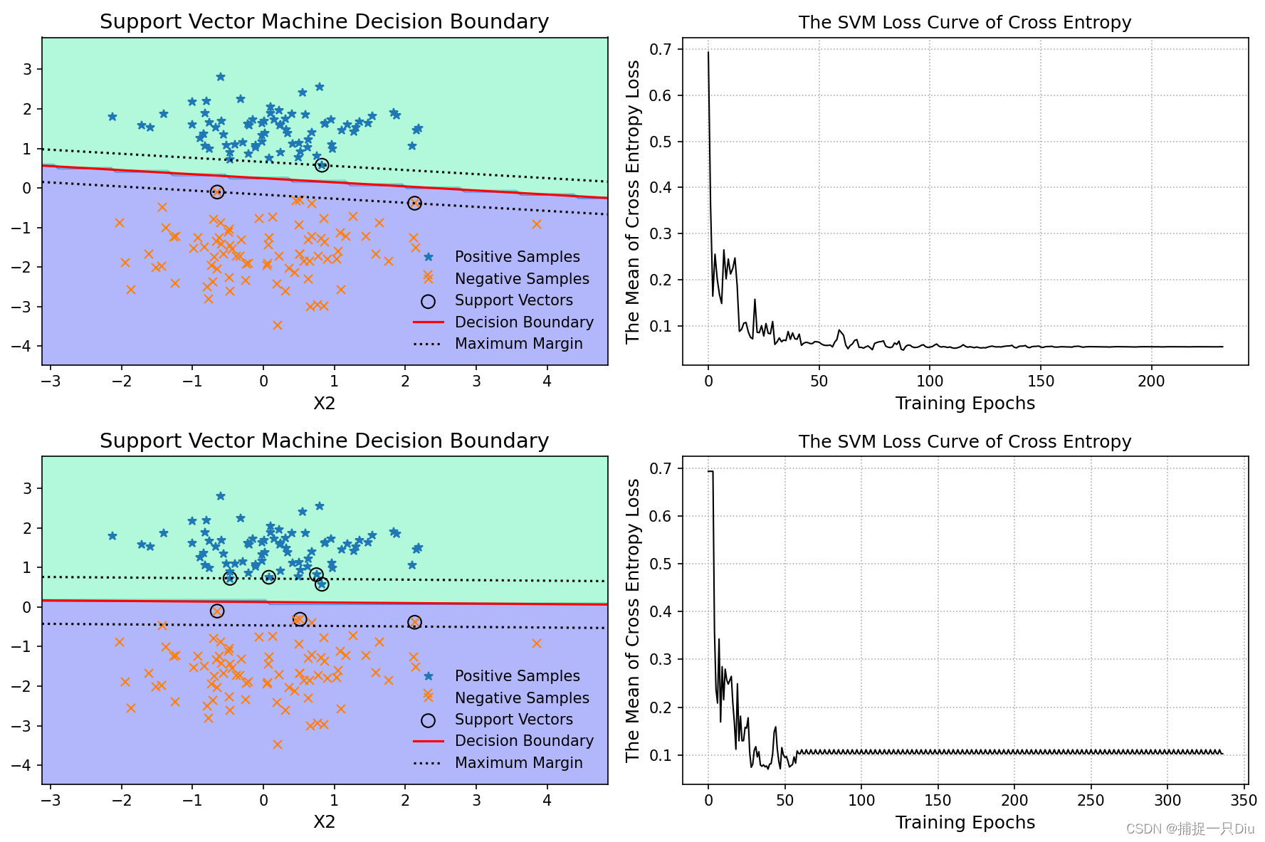
# C = 1000，倾向于硬间隔
svm = SVMClassifier(C=1000)
svm.fit(X_train, y_train)
y_test_pred = svm.predict(X_test)
print(classification_report(y_test, y_test_pred))

plt.figure(figsize=(14, 10))
plt.subplot(221)
svm.plt_svm(X_train, y_train, is_show=False, is_margin=True)
plt.subplot(222)
svm.plt_loss_curve(is_show=False)

# C = 1，倾向于软间隔
svm = SVMClassifier(C=1)
svm.fit(X_train, y_train)
y_test_pred = svm.predict(X_test)
print(classification_report(y_test, y_test_pred))

plt.subplot(223)
svm.plt_svm(X_train, y_train, is_show=False, is_margin=True)
plt.subplot(224)
svm.plt_loss_curve(is_show=False)

plt.tight_layout()
plt.show()

 test_svm_kernel_classifier.py 

import numpy as np
import matplotlib.pyplot as plt
from sklearn.datasets import make_classification, make_moons
from sklearn.model_selection import train_test_split
from svm_smo_classifier import SVMClassifier
from sklearn.metrics import classification_report


X, y = make_moons(n_samples=200, noise=0.1)
X_train, X_test, y_train, y_test = train_test_split(X, y, test_size=0.2, random_state=0, shuffle=True)

svm_rbf = SVMClassifier(C=10.0, kernel="rbf", gamma=0.5)
svm_rbf.fit(X_train, y_train)
y_test_pred = svm_rbf.predict(X_test)
print(classification_report(y_test, y_test_pred))
print("=" * 60)
svm_poly = SVMClassifier(C=10.0, kernel="poly", degree=3)
svm_poly.fit(X_train, y_train)
y_test_pred = svm_poly.predict(X_test)
print(classification_report(y_test, y_test_pred))

plt.figure(figsize=(14, 10))
plt.subplot(221)
svm_rbf.plt_svm(X_train, y_train, is_show=False)
plt.subplot(222)
svm_rbf.plt_loss_curve(is_show=False)

plt.subplot(223)
svm_poly.plt_svm(X_train, y_train, is_show=False)
plt.subplot(224)
svm_poly.plt_loss_curve(is_show=False)

plt.tight_layout()
plt.show()

 test_svm_kernel_classifier2.py 

import numpy as np
import matplotlib.pyplot as plt
from sklearn.datasets import make_classification, make_moons
from sklearn.model_selection import train_test_split
from svm_smo_classifier import SVMClassifier
from sklearn.metrics import classification_report


X, y = make_classification(n_samples=100, n_features=2, n_classes=2, n_informative=1,
                           n_redundant=0, n_repeated=0, n_clusters_per_class=1,
                           class_sep=0.8, random_state=21)
X_train, X_test, y_train, y_test = train_test_split(X, y, test_size=0.2, random_state=0, shuffle=True)

svm_rbf1 = SVMClassifier(C=10.0, kernel="rbf", gamma=0.1)
svm_rbf1.fit(X_train, y_train)
y_test_pred = svm_rbf1.predict(X_test)
print(classification_report(y_test, y_test_pred))
print("=" * 60)
svm_rbf2 = SVMClassifier(C=1.0, kernel="rbf", gamma=0.5)
svm_rbf2.fit(X_train, y_train)
y_test_pred = svm_rbf2.predict(X_test)
print(classification_report(y_test, y_test_pred))
print("=" * 60)

svm_poly1 = SVMClassifier(C=10.0, kernel="poly", degree=3)
svm_poly1.fit(X_train, y_train)
y_test_pred = svm_poly1.predict(X_test)
print(classification_report(y_test, y_test_pred))
svm_poly2 = SVMClassifier(C=10.0, kernel="poly", degree=6)
svm_poly2.fit(X_train, y_train)
y_test_pred = svm_poly2.predict(X_test)
print(classification_report(y_test, y_test_pred))

X, y = make_classification(n_samples=100, n_features=2, n_classes=2, n_informative=1,
                           n_redundant=0, n_repeated=0, n_clusters_per_class=1,
                           class_sep=0.8, random_state=21)
X_train1, X_test1, y_train1, y_test1 = train_test_split(X, y, test_size=0.2, random_state=0, shuffle=True)

svm_linear1 = SVMClassifier(C=10.0, kernel="linear")
svm_linear1.fit(X_train1, y_train1)
y_test_pred1 = svm_linear1.predict(X_test1)
print(classification_report(y_test1, y_test_pred1))
svm_linear2 = SVMClassifier(C=10.0, kernel="linear")
svm_linear2.fit(X_train1, y_train1)
y_test_pred = svm_linear2.predict(X_test1)
print(classification_report(y_test1, y_test_pred1))

plt.figure(figsize=(21, 10))
plt.subplot(231)
svm_rbf1.plt_svm(X_train, y_train, is_show=False)
plt.subplot(232)
svm_rbf2.plt_svm(X_train, y_train, is_show=False)
plt.subplot(233)
svm_poly1.plt_svm(X_train, y_train, is_show=False)
plt.subplot(234)
svm_poly2.plt_svm(X_train, y_train, is_show=False)
plt.subplot(235)
svm_linear1.plt_svm(X_train1, y_train1, is_show=False, is_margin=True)
plt.subplot(236)
svm_linear2.plt_svm(X_train1, y_train1, is_show=False, is_margin=True)

plt.tight_layout()
plt.show()