


│ ├─Maize
│ ├─Scentless Mayweed
│ ├─Shepherds Purse
│ ├─Small-flowered Cranesbill
│ └─Sugar beet
├─train.py
├─test1.py
└─test.py
=============================================================
新建train.py
import numpy as np
from tensorflow.keras.optimizers import Adam
import cv2
from tensorflow.keras.preprocessing.image import img_to_array
from sklearn.model_selection import train_test_split
from tensorflow.python.keras.callbacks import ModelCheckpoint, ReduceLROnPlateau
from tensorflow.keras.applications import MobileNetV2
import os
from tensorflow.python.keras.layers import Dense
from tensorflow.python.keras.models import Sequential
import albumentations
norm_size = 224
datapath = ‘data/train’
EPOCHS = 100
INIT_LR = 1e-3
labelList = []
dicClass = {‘Black-grass’: 0, ‘Charlock’: 1, ‘Cleavers’: 2, ‘Common Chickweed’: 3, ‘Common wheat’: 4, ‘Fat Hen’: 5, ‘Loose Silky-bent’: 6,
‘Maize’: 7, ‘Scentless Mayweed’: 8, ‘Shepherds Purse’: 9, ‘Small-flowered Cranesbill’: 10, ‘Sugar beet’: 11}
classnum = 12
batch_size = 16
np.random.seed(42)
这里可以看出tensorflow2.0以上的版本集成了Keras,我们在使用的时候就不必单独安装Keras了,以前的代码升级到tensorflow2.0以上的版本将keras前面加上tensorflow即可。
tensorflow说完了,再说明一下几个重要的全局参数:
-
norm_size = 224, 设置输入图像的大小,MobileNetV2默认的图片尺寸是224×224。
-
datapath = ‘data/train’, 设置图片存放的路径,在这里要说明一下如果图片很多,一定不要放在工程目录下,否则Pycharm加载工程的时候会浏览所有的图片,很慢很慢。
-
EPOCHS = 100, epochs的数量,关于epoch的设置多少合适,这个问题很纠结,一般情况设置300足够了,如果感觉没有训练好,再载入模型训练。
-
INIT_LR = 1e-3, 学习率,一般情况从0.001开始逐渐降低,也别太小了到1e-6就可以了。
-
classnum = 12, 类别数量,数据集有两个类别,所有就分为两类。
-
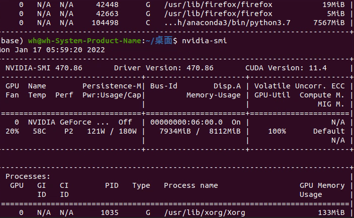
batch_size =16, batchsize,根据硬件的情况和数据集的大小设置,太小了loss浮动太大,太大了收敛不好,根据经验来,一般设置为2的次方。windows可以通过任务管理器查看显存的占用情况。

Ubuntu可以使用nvidia-smi查看显存的占用。
- 定义numpy.random的随机因子。这样就可以固定随机的index
和以前做法不同的是,这里不再处理图片,而是只返回图片路径的list列表。
具体做法详见代码:
def loadImageData():
imageList = []
listClasses = os.listdir(datapath) # 类别文件夹
print(listClasses)
for class_name in listClasses:
label_id = dicClass[class_name]
class_path = os.path.join(datapath, class_name)
image_names = os.listdir(class_path)
for image_name in image_names:
image_full_path = os.path.join(class_path, image_name)
labelList.append(label_id)
imageList.append(image_full_path)
return imageList
print(“开始加载数据”)
imageArr = loadImageData()
labelList = np.array(labelList)
print(“加载数据完成”)
print(labelList)
做好数据之后,我们需要切分训练集和测试集,一般按照4:1或者7:3的比例来切分。切分数据集使用train_test_split()方法,需要导入from sklearn.model_selection import train_test_split 包。例:
trainX, valX, trainY, valY = train_test_split(imageArr, labelList, test_size=0.2, random_state=42)
train_transform = albumentations.Compose([
albumentations.OneOf([
albumentations.RandomGamma(gamma_limit=(60, 120), p=0.9),
albumentations.RandomBrightnessContrast(brightness_limit=0.2, contrast_limit=0.2, p=0.9),
albumentations.CLAHE(clip_limit=4.0, tile_grid_size=(4, 4), p=0.9),
]),
albumentations.HorizontalFlip(p=0.5),
albumentations.ShiftScaleRotate(shift_limit=0.2, scale_limit=0.2, rotate_limit=20,
interpolation=cv2.INTER_LINEAR, border_mode=cv2.BORDER_CONSTANT, p=1),
albumentations.Normalize(mean=(0.485, 0.456, 0.406), std=(0.229, 0.224, 0.225), max_pixel_value=255.0, p=1.0)
])
val_transform = albumentations.Compose([
albumentations.Normalize(mean=(0.485, 0.456, 0.406), std=(0.229, 0.224, 0.225), max_pixel_value=255.0, p=1.0)
])
这个随意写的,具体的设置可以参考我以前写的文章:
图像增强库Albumentations使用总结_AI浩-CSDN博客_albumentations
写了两个数据增强,一个是用于训练,一个用于验证。验证集只需要对图片做归一化处理。
generator的主要作用是处理图像,并迭代的方式返回一个batch的图像以及对应的label。
思路:
在while循环:
-
初始化input_samples和input_labels,连个list分别用来存放image和image对应的标签。
-
循环batch_size次数:
-
- 随机一个index
-
分别从file_pathList和labels,得到图片的路径和对应的label
-
读取图片
-
如果是训练就训练的transform,如果不是就执行验证的transform。
-
resize图片
-
将image转数组
-
将图像和label分别放到input_samples和input_labels
-
将list转numpy数组。
-
返回一次迭代
def generator(file_pathList,labels,batch_size,train_action=False):
L = len(file_pathList)
while True:
input_labels = []
input_samples = []
for row in range(0, batch_size):
temp = np.random.randint(0, L)
X = file_pathList[temp]
Y = labels[temp]
image = cv2.imdecode(np.fromfile(X, dtype=np.uint8), -1)
if image.shape[2] > 3:
image = image[:, :, :3]
if train_action:
image=train_transform(image=image)[‘image’]
else:
image = val_transform(image=image)[‘image’]
image = cv2.resize(image, (norm_size, norm_size), interpolation=cv2.INTER_LANCZOS4)
image = img_to_array(image)
input_samples.append(image)
input_labels.append(Y)
batch_x = np.asarray(input_samples)
batch_y = np.asarray(input_labels)
yield (batch_x, batch_y)
ModelCheckpoint:用来保存成绩最好的模型。
语法如下:
keras.callbacks.ModelCheckpoint(filepath, monitor=‘val_loss’, verbose=0, save_best_only=False, save_weights_only=False, mode=‘auto’, period=1)
该回调函数将在每个epoch后保存模型到filepath
filepath可以是格式化的字符串,里面的占位符将会被epoch值和传入on_epoch_end的logs关键字所填入
例如,filepath若为weights.{epoch:02d-{val_loss:.2f}}.hdf5,则会生成对应epoch和验证集loss的多个文件。
参数
- filename:字符串,保存模型的路径
- monitor:需要监视的值
- verbose:信息展示模式,0或1
- save_best_only:当设置为True时,将只保存在验证集上性能最好的模型
- mode:‘auto’,‘min’,‘max’之一,在save_best_only=True时决定性能最佳模型的评判准则,例如,当监测值为val_acc时,模式应为max,当检测值为val_loss时,模式应为min。在auto模式下,评价准则由被监测值的名字自动推断。
- save_weights_only:若设置为True,则只保存模型权重,否则将保存整个模型(包括模型结构,配置信息等)
- period:CheckPoint之间的间隔的epoch数
ReduceLROnPlateau:当评价指标不在提升时,减少学习率,语法如下:
keras.callbacks.ReduceLROnPlateau(monitor=‘val_loss’, factor=0.1, patience=10, verbose=0, mode=‘auto’, epsilon=0.0001, cooldown=0, min_lr=0)
当学习停滞时,减少2倍或10倍的学习率常常能获得较好的效果。该回调函数检测指标的情况,如果在patience个epoch中看不到模型性能提升,则减少学习率
参数
- monitor:被监测的量
- factor:每次减少学习率的因子,学习率将以lr = lr*factor的形式被减少
- patience:当patience个epoch过去而模型性能不提升时,学习率减少的动作会被触发
- mode:‘auto’,‘min’,‘max’之一,在min模式下,如果检测值触发学习率减少。在max模式下,当检测值不再上升则触发学习率减少。
- epsilon:阈值,用来确定是否进入检测值的“平原区”
- cooldown:学习率减少后,会经过cooldown个epoch才重新进行正常操作
- min_lr:学习率的下限
本例代码如下:
checkpointer = ModelCheckpoint(filepath=‘best_model.hdf5’,
monitor=‘val_accuracy’, verbose=1, save_best_only=True, mode=‘max’)
reduce = ReduceLROnPlateau(monitor=‘val_accuracy’, patience=10,
verbose=1,
factor=0.5,
min_lr=1e-6)
model = Sequential()
model.add(MobileNetV2(include_top=False, pooling=‘avg’, weights=‘imagenet’))
model.add(Dense(classnum, activation=‘softmax’))
optimizer = Adam(learning_rate=INIT_LR)
model.compile(optimizer=optimizer, loss=‘sparse_categorical_crossentropy’, metrics=[‘accuracy’])
history = model.fit(generator(trainX,trainY,batch_size,train_action=True),
steps_per_epoch=len(trainX) / batch_size,
validation_data=generator(valX,valY,batch_size,train_action=False),
epochs=EPOCHS,
validation_steps=len(valX) / batch_size,
callbacks=[checkpointer, reduce])
model.save(‘my_model.h5’)
print(history)
如果想指定classes,有两个条件:include_top:True, weights:None。否则无法指定classes。
所以指定classes就不能用预训练了,所以采用另一种方式:
model = Sequential()
model.add(MobileNet(include_top=False, pooling=‘avg’, weights=‘imagenet’))
model.add(Dense(classnum, activation=‘softmax’))
这样既能使用预训练,又能指定classnum。
另外,在2.X版本中fit支持generator方式,所以直接使用fit。
loss_trend_graph_path = r"WW_loss.jpg"
acc_trend_graph_path = r"WW_acc.jpg"
import matplotlib.pyplot as plt
print(“Now,we start drawing the loss and acc trends graph…”)
summarize history for accuracy
fig = plt.figure(1)
plt.plot(history.history[“accuracy”])
plt.plot(history.history[“val_accuracy”])
plt.title(“Model accuracy”)
plt.ylabel(“accuracy”)
plt.xlabel(“epoch”)
plt.legend([“train”, “test”], loc=“upper left”)
网上学习资料一大堆,但如果学到的知识不成体系,遇到问题时只是浅尝辄止,不再深入研究,那么很难做到真正的技术提升。
一个人可以走的很快,但一群人才能走的更远!不论你是正从事IT行业的老鸟或是对IT行业感兴趣的新人,都欢迎加入我们的的圈子(技术交流、学习资源、职场吐槽、大厂内推、面试辅导),让我们一起学习成长!
h…")
summarize history for accuracy
fig = plt.figure(1)
plt.plot(history.history[“accuracy”])
plt.plot(history.history[“val_accuracy”])
plt.title(“Model accuracy”)
plt.ylabel(“accuracy”)
plt.xlabel(“epoch”)
plt.legend([“train”, “test”], loc=“upper left”)
[外链图片转存中…(img-gOG8UjGg-1714669607922)]
[外链图片转存中…(img-yiB4Keml-1714669607922)]
网上学习资料一大堆,但如果学到的知识不成体系,遇到问题时只是浅尝辄止,不再深入研究,那么很难做到真正的技术提升。
一个人可以走的很快,但一群人才能走的更远!不论你是正从事IT行业的老鸟或是对IT行业感兴趣的新人,都欢迎加入我们的的圈子(技术交流、学习资源、职场吐槽、大厂内推、面试辅导),让我们一起学习成长!


 2300
2300


 被折叠的 条评论
为什么被折叠?
被折叠的 条评论
为什么被折叠?
 到【灌水乐园】发言


