Python基础（十三） 机器学习sklearn库详解与应用_e anad lib site-packages sklearn linear_model _lo(1)

既有适合小白学习的零基础资料，也有适合3年以上经验的小伙伴深入学习提升的进阶课程，涵盖了95%以上Go语言开发知识点，真正体系化！

由于文件比较多，这里只是将部分目录截图出来，全套包含大厂面经、学习笔记、源码讲义、实战项目、大纲路线、讲解视频，并且后续会持续更新

如果你需要这些资料，可以戳这里获取

iris.head()

	sepal_length	sepal_width	petal_length	petal_width	species
0	5.1	3.5	1.4	0.2	setosa
1	4.9	3.0	1.4	0.2	setosa
2	4.7	3.2	1.3	0.2	setosa
3	4.6	3.1	1.5	0.2	setosa
4	5.0	3.6	1.4	0.2	setosa

iris.info()

<class 'pandas.core.frame.DataFrame'>
RangeIndex: 150 entries, 0 to 149
Data columns (total 5 columns):
 #   Column        Non-Null Count  Dtype  
---  ------        --------------  -----  
 0   sepal_length  150 non-null    float64
 1   sepal_width   150 non-null    float64
 2   petal_length  150 non-null    float64
 3   petal_width   150 non-null    float64
 4   species       150 non-null    object 
dtypes: float64(4), object(1)
memory usage: 6.0+ KB

iris.describe()

	sepal_length	sepal_width	petal_length	petal_width
count	150.000000	150.000000	150.000000	150.000000
mean	5.843333	3.057333	3.758000	1.199333
std	0.828066	0.435866	1.765298	0.762238
min	4.300000	2.000000	1.000000	0.100000
25%	5.100000	2.800000	1.600000	0.300000
50%	5.800000	3.000000	4.350000	1.300000
75%	6.400000	3.300000	5.100000	1.800000
max	7.900000	4.400000	6.900000	2.500000

iris.species.value_counts()

virginica     50
versicolor    50
setosa        50
Name: species, dtype: int64

sns.pairplot(data=iris, hue="species")

<seaborn.axisgrid.PairGrid at 0x178f9d81160>

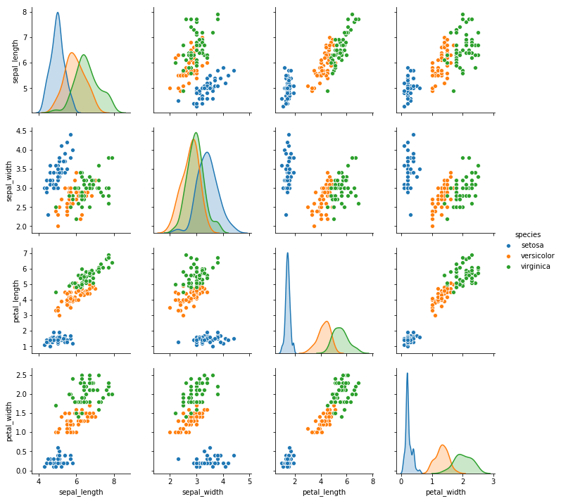
可见，花瓣的长度和宽度有非常好的相关性。而花萼的长宽效果不好，因此考虑对他们丢弃。

【3】数据清洗

iris_simple = iris.drop(["sepal\_length", "sepal\_width"], axis=1)
iris_simple.head()

	petal_length	petal_width	species
0	1.4	0.2	setosa
1	1.4	0.2	setosa
2	1.3	0.2	setosa
3	1.5	0.2	setosa
4	1.4	0.2	setosa

【4】标签编码

from sklearn.preprocessing import LabelEncoder

encoder = LabelEncoder()
iris_simple["species"] = encoder.fit_transform(iris_simple["species"])

iris_simple

	petal_length	petal_width	species
0	1.4	0.2	0
1	1.4	0.2	0
2	1.3	0.2	0
3	1.5	0.2	0
4	1.4	0.2	0
5	1.7	0.4	0
6	1.4	0.3	0
7	1.5	0.2	0
8	1.4	0.2	0
9	1.5	0.1	0
10	1.5	0.2	0
11	1.6	0.2	0
12	1.4	0.1	0
13	1.1	0.1	0
14	1.2	0.2	0
15	1.5	0.4	0
16	1.3	0.4	0
17	1.4	0.3	0
18	1.7	0.3	0
19	1.5	0.3	0
20	1.7	0.2	0
21	1.5	0.4	0
22	1.0	0.2	0
23	1.7	0.5	0
24	1.9	0.2	0
25	1.6	0.2	0
26	1.6	0.4	0
27	1.5	0.2	0
28	1.4	0.2	0
29	1.6	0.2	0
…	…	…	…
120	5.7	2.3	2
121	4.9	2.0	2
122	6.7	2.0	2
123	4.9	1.8	2
124	5.7	2.1	2
125	6.0	1.8	2
126	4.8	1.8	2
127	4.9	1.8	2
128	5.6	2.1	2
129	5.8	1.6	2
130	6.1	1.9	2
131	6.4	2.0	2
132	5.6	2.2	2
133	5.1	1.5	2
134	5.6	1.4	2
135	6.1	2.3	2
136	5.6	2.4	2
137	5.5	1.8	2
138	4.8	1.8	2
139	5.4	2.1	2
140	5.6	2.4	2
141	5.1	2.3	2
142	5.1	1.9	2
143	5.9	2.3	2
144	5.7	2.5	2
145	5.2	2.3	2
146	5.0	1.9	2
147	5.2	2.0	2
148	5.4	2.3	2
149	5.1	1.8	2

150 rows × 3 columns

【5】数据集的标准化（本数据集特征比较接近，实际处理过程中未标准化）

from sklearn.preprocessing import StandardScaler
import pandas as pd

trans = StandardScaler()
_iris_simple = trans.fit_transform(iris_simple[["petal\_length", "petal\_width"]])
_iris_simple = pd.DataFrame(_iris_simple, columns = ["petal\_length", "petal\_width"])
_iris_simple.describe()

	petal_length	petal_width
count	1.500000e+02	1.500000e+02
mean	-8.652338e-16	-4.662937e-16
std	1.003350e+00	1.003350e+00
min	-1.567576e+00	-1.447076e+00
25%	-1.226552e+00	-1.183812e+00
50%	3.364776e-01	1.325097e-01
75%	7.627583e-01	7.906707e-01
max	1.785832e+00	1.712096e+00

【6】构建训练集和测试集（本课暂不考虑验证集）

from sklearn.model_selection import train_test_split

train_set, test_set = train_test_split(iris_simple, test_size=0.2) # 20%的数据作为测试集
test_set.head()

	petal_length	petal_width	species
3	1.5	0.2	0
111	5.3	1.9	2
24	1.9	0.2	0
5	1.7	0.4	0
92	4.0	1.2	1

iris_x_train = train_set[["petal\_length", "petal\_width"]]
iris_x_train.head()

	petal_length	petal_width
63	4.7	1.4
93	3.3	1.0
34	1.5	0.2
35	1.2	0.2
126	4.8	1.8

iris_y_train = train_set["species"].copy()
iris_y_train.head()

63     1
93     1
34     0
35     0
126    2
Name: species, dtype: int32

iris_x_test = test_set[["petal\_length", "petal\_width"]]
iris_x_test.head()

	petal_length	petal_width
3	1.5	0.2
111	5.3	1.9
24	1.9	0.2
5	1.7	0.4
92	4.0	1.2

iris_y_test = test_set["species"].copy()
iris_y_test.head()

3      0
111    2
24     0
5      0
92     1
Name: species, dtype: int32

13.1 k近邻算法

【1】基本思想

与待预测点最近的训练数据集中的k个邻居

把k个近邻中最常见的类别预测为带预测点的类别

【2】sklearn实现

from sklearn.neighbors import KNeighborsClassifier

• 构建分类器对象

clf = KNeighborsClassifier()
clf

KNeighborsClassifier(algorithm='auto', leaf_size=30, metric='minkowski',
                     metric_params=None, n_jobs=None, n_neighbors=5, p=2,
                     weights='uniform')

• 训练

clf.fit(iris_x_train, iris_y_train)

KNeighborsClassifier(algorithm='auto', leaf_size=30, metric='minkowski',
                     metric_params=None, n_jobs=None, n_neighbors=5, p=2,
                     weights='uniform')

• 预测

res = clf.predict(iris_x_test)
print(res)
print(iris_y_test.values)

[0 2 0 0 1 1 0 2 1 2 1 2 2 2 1 0 0 0 1 0 2 0 2 1 0 1 0 0 1 1]
[0 2 0 0 1 1 0 2 2 2 1 2 2 2 1 0 0 0 1 0 2 0 2 1 0 1 0 0 1 1]

• 翻转

encoder.inverse_transform(res)

array(['setosa', 'virginica', 'setosa', 'setosa', 'versicolor',
       'versicolor', 'setosa', 'virginica', 'versicolor', 'virginica',
       'versicolor', 'virginica', 'virginica', 'virginica', 'versicolor',
       'setosa', 'setosa', 'setosa', 'versicolor', 'setosa', 'virginica',
       'setosa', 'virginica', 'versicolor', 'setosa', 'versicolor',
       'setosa', 'setosa', 'versicolor', 'versicolor'], dtype=object)

• 评估

accuracy = clf.score(iris_x_test, iris_y_test)
print("预测正确率:{:.0%}".format(accuracy))

预测正确率:97%

• 存储数据

out = iris_x_test.copy()
out["y"] = iris_y_test
out["pre"] = res
out

	petal_length	petal_width	y	pre
3	1.5	0.2	0	0
111	5.3	1.9	2	2
24	1.9	0.2	0	0
5	1.7	0.4	0	0
92	4.0	1.2	1	1
57	3.3	1.0	1	1
1	1.4	0.2	0	0
112	5.5	2.1	2	2
106	4.5	1.7	2	1
136	5.6	2.4	2	2
80	3.8	1.1	1	1
131	6.4	2.0	2	2
147	5.2	2.0	2	2
113	5.0	2.0	2	2
84	4.5	1.5	1	1
39	1.5	0.2	0	0
40	1.3	0.3	0	0
17	1.4	0.3	0	0
56	4.7	1.6	1	1
2	1.3	0.2	0	0
100	6.0	2.5	2	2
42	1.3	0.2	0	0
144	5.7	2.5	2	2
79	3.5	1.0	1	1
19	1.5	0.3	0	0
75	4.4	1.4	1	1
44	1.9	0.4	0	0
37	1.4	0.1	0	0
64	3.6	1.3	1	1
90	4.4	1.2	1	1

out.to_csv("iris\_predict.csv")

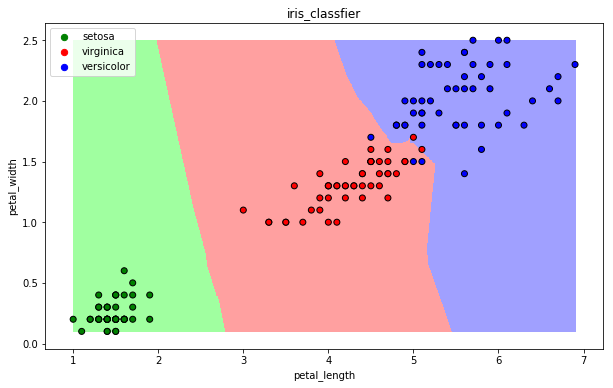
【3】可视化

import numpy as np
import matplotlib as mpl
import matplotlib.pyplot as plt

def draw(clf):

    # 网格化
    M, N = 500, 500
    x1_min, x2_min = iris_simple[["petal\_length", "petal\_width"]].min(axis=0)
    x1_max, x2_max = iris_simple[["petal\_length", "petal\_width"]].max(axis=0)
    t1 = np.linspace(x1_min, x1_max, M)
    t2 = np.linspace(x2_min, x2_max, N)
    x1, x2 = np.meshgrid(t1, t2)
    
    # 预测
    x_show = np.stack((x1.flat, x2.flat), axis=1)
    y_predict = clf.predict(x_show)
    
    # 配色
    cm_light = mpl.colors.ListedColormap(["#A0FFA0", "#FFA0A0", "#A0A0FF"])
    cm_dark = mpl.colors.ListedColormap(["g", "r", "b"])
    
    # 绘制预测区域图
    plt.figure(figsize=(10, 6))
    plt.pcolormesh(t1, t2, y_predict.reshape(x1.shape), cmap=cm_light)
    
    # 绘制原始数据点
    plt.scatter(iris_simple["petal\_length"], iris_simple["petal\_width"], label=None,
                c=iris_simple["species"], cmap=cm_dark, marker='o', edgecolors='k')
    plt.xlabel("petal\_length")
    plt.ylabel("petal\_width")
    
    # 绘制图例
    color = ["g", "r", "b"]
    species = ["setosa", "virginica", "versicolor"]
    for i in range(3):
        plt.scatter([], [], c=color[i], s=40, label=species[i])    # 利用空点绘制图例
    plt.legend(loc="best")
    plt.title('iris\_classfier')

draw(clf)

13.2 朴素贝叶斯算法

【1】基本思想

当X=(x1, x2)发生的时候，哪一个yk发生的概率最大

【2】sklearn实现

from sklearn.naive_bayes import GaussianNB

• 构建分类器对象

clf = GaussianNB()
clf

• 训练

clf.fit(iris_x_train, iris_y_train)

• 预测

res = clf.predict(iris_x_test)
print(res)
print(iris_y_test.values)

[0 2 0 0 1 1 0 2 1 2 1 2 2 2 1 0 0 0 1 0 2 0 2 1 0 1 0 0 1 1]
[0 2 0 0 1 1 0 2 2 2 1 2 2 2 1 0 0 0 1 0 2 0 2 1 0 1 0 0 1 1]

• 评估

accuracy = clf.score(iris_x_test, iris_y_test)
print("预测正确率:{:.0%}".format(accuracy))

预测正确率:97%

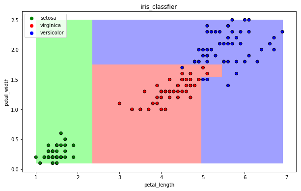
• 可视化

draw(clf)

13.3 决策树算法

【1】基本思想

CART算法：每次通过一个特征，将数据尽可能的分为纯净的两类，递归的分下去

【2】sklearn实现

from sklearn.tree import DecisionTreeClassifier

• 构建分类器对象

clf = DecisionTreeClassifier()
clf

DecisionTreeClassifier(class_weight=None, criterion='gini', max_depth=None,
                       max_features=None, max_leaf_nodes=None,
                       min_impurity_decrease=0.0, min_impurity_split=None,
                       min_samples_leaf=1, min_samples_split=2,
                       min_weight_fraction_leaf=0.0, presort=False,
                       random_state=None, splitter='best')

• 训练

clf.fit(iris_x_train, iris_y_train)

DecisionTreeClassifier(class_weight=None, criterion='gini', max_depth=None,
                       max_features=None, max_leaf_nodes=None,
                       min_impurity_decrease=0.0, min_impurity_split=None,
                       min_samples_leaf=1, min_samples_split=2,
                       min_weight_fraction_leaf=0.0, presort=False,
                       random_state=None, splitter='best')

• 预测

res = clf.predict(iris_x_test)
print(res)
print(iris_y_test.values)

[0 2 0 0 1 1 0 2 1 2 1 2 2 2 1 0 0 0 1 0 2 0 2 1 0 1 0 0 1 1]
[0 2 0 0 1 1 0 2 2 2 1 2 2 2 1 0 0 0 1 0 2 0 2 1 0 1 0 0 1 1]

• 评估

accuracy = clf.score(iris_x_test, iris_y_test)
print("预测正确率:{:.0%}".format(accuracy))

预测正确率:97%

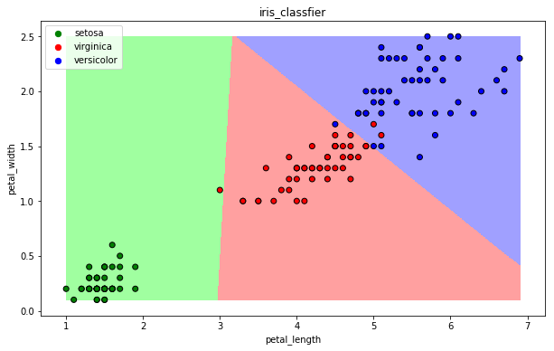
• 可视化

draw(clf)

13.4 逻辑回归算法

【1】基本思想

一种解释：

训练：通过一个映射方式，将特征X=（x1, x2） 映射成 P(y=ck), 求使得所有概率之积最大化的映射方式里的参数

预测：计算p(y=ck) 取概率最大的那个类别作为预测对象的分类

【2】sklearn实现

from sklearn.linear_model import LogisticRegression

• 构建分类器对象

clf = LogisticRegression(solver='saga', max_iter=1000)
clf

LogisticRegression(C=1.0, class_weight=None, dual=False, fit_intercept=True,
                   intercept_scaling=1, l1_ratio=None, max_iter=1000,
                   multi_class='warn', n_jobs=None, penalty='l2',
                   random_state=None, solver='saga', tol=0.0001, verbose=0,
                   warm_start=False)

• 训练

clf.fit(iris_x_train, iris_y_train)

C:\Users\ibm\Anaconda3\lib\site-packages\sklearn\linear_model\logistic.py:469: FutureWarning: Default multi_class will be changed to 'auto' in 0.22. Specify the multi_class option to silence this warning.
  "this warning.", FutureWarning)





LogisticRegression(C=1.0, class_weight=None, dual=False, fit_intercept=True,
                   intercept_scaling=1, l1_ratio=None, max_iter=1000,
                   multi_class='warn', n_jobs=None, penalty='l2',
                   random_state=None, solver='saga', tol=0.0001, verbose=0,
                   warm_start=False)

• 预测

res = clf.predict(iris_x_test)
print(res)
print(iris_y_test.values)

[0 2 0 0 1 1 0 2 1 2 1 2 2 2 1 0 0 0 1 0 2 0 2 1 0 1 0 0 1 1]
[0 2 0 0 1 1 0 2 2 2 1 2 2 2 1 0 0 0 1 0 2 0 2 1 0 1 0 0 1 1]

• 评估

accuracy = clf.score(iris_x_test, iris_y_test)
print("预测正确率:{:.0%}".format(accuracy))

预测正确率:97%

• 可视化

draw(clf)

13.5 支持向量机算法

既有适合小白学习的零基础资料，也有适合3年以上经验的小伙伴深入学习提升的进阶课程，涵盖了95%以上Go语言开发知识点，真正体系化！

由于文件比较多，这里只是将部分目录截图出来，全套包含大厂面经、学习笔记、源码讲义、实战项目、大纲路线、讲解视频，并且后续会持续更新

如果你需要这些资料，可以戳这里获取

* 预测

res = clf.predict(iris_x_test)
print(res)
print(iris_y_test.values)

[0 2 0 0 1 1 0 2 1 2 1 2 2 2 1 0 0 0 1 0 2 0 2 1 0 1 0 0 1 1]
[0 2 0 0 1 1 0 2 2 2 1 2 2 2 1 0 0 0 1 0 2 0 2 1 0 1 0 0 1 1]

* 评估

accuracy = clf.score(iris_x_test, iris_y_test)
print(“预测正确率:{:.0%}”.format(accuracy))

预测正确率:97%

* 可视化

draw(clf)

![image-20221003185357659](https://img-blog.csdnimg.cn/img_convert/70b0e796eb05f176620879d79064ed65.png)


### 13.5 支持向量机算法



[外链图片转存中...(img-nSWma77I-1715907962183)]
[外链图片转存中...(img-0E13TDhG-1715907962184)]
[外链图片转存中...(img-EQjb5DgB-1715907962184)]

**既有适合小白学习的零基础资料，也有适合3年以上经验的小伙伴深入学习提升的进阶课程，涵盖了95%以上Go语言开发知识点，真正体系化！**

**由于文件比较多，这里只是将部分目录截图出来，全套包含大厂面经、学习笔记、源码讲义、实战项目、大纲路线、讲解视频，并且后续会持续更新**

**[如果你需要这些资料，可以戳这里获取](https://bbs.csdn.net/topics/618658159)**