


OR-Tools 解决的问题类型:
线性优化示例
线性优化(或线性规划)是最古老且使用最广泛的优化领域之一,其中目标函数和约束可以写为线性表达式。
在以下约束下最大化3x + y:
| 0 | ≤ | x | ≤ | 1 |
| 0 | ≤ | y | ≤ | 2 |
| x + y | ≤ | 2 |
目标函数为3x + y。 目标函数和约束都由线性表达式给出,这使它成为线性问题。
 def eg_linear():
    # 3x+y,0<=x<=1,0<=y<=2,x+y<=2
    # libraries
    from ortools.linear_solver import pywraplp
    # Create the linear solver with the GLOP backend.
    solver = pywraplp.Solver.CreateSolver('simple_lp_program', 'GLOP')
    # Create the variables x and y.
    x = solver.NumVar(0, 1, 'x')
    y = solver.NumVar(0, 2, 'y')
    print('Number of variables =', solver.NumVariables())
    # Create a linear constraint, 0 <= x + y <= 2.
    ct = solver.Constraint(0, 2, 'ct')
    ct.SetCoefficient(x, 1)
    ct.SetCoefficient(y, 1)

    print('Number of constraints =', solver.NumConstraints())
    # Create the objective function, 3 * x + y.
    objective = solver.Objective()
    objective.SetCoefficient(x, 3)
    objective.SetCoefficient(y, 1)
    objective.SetMaximization()
    solver.Solve()
    print('Solution:')
    print('Objective value =', objective.Value())
    print('x =', x.solution_value())
    print('y =', y.solution_value())
整数优化:
某些变量为整数的线性优化问题称为混合整数程序(MIPs)。这些变量可以通过以下几种方式出现:
- 表示项目数(如汽车或电视机)的整数变量,问题是决定要制造的每个物料中有多少件,以便实现利润最大化。通常,此类问题可以设置为标准线性优化问题,并附加要求变量必须为整数。
- 表示具有 0-1值的决策的布尔变量。例如,考虑一个涉及将工作人员分配给任务的问题。若要设置这种类型的问题,可以定义布尔变量xi,j 等于 1(如果辅助角色 i 分配给任务 j),否则为 0。
例子:目标最大化x = 10y
| x = 7 y | ≤ | 17.5 |
| Ⅹ | ≤ | 3.5 |
| Ⅹ | ≥ | 0 |
| Y | ≥ | 0 |
| x, y整数 | ||
from __future__ import print_function
from ortools.linear_solver import pywraplp


def main():
    # Create the mip solver with the CBC backend.
    solver = pywraplp.Solver.CreateSolver('simple_mip_program', 'CBC')

    infinity = solver.infinity()
    # x and y are integer non-negative variables.
    x = solver.IntVar(0.0, infinity, 'x')
    y = solver.IntVar(0.0, infinity, 'y')

    print('Number of variables =', solver.NumVariables())

    # x + 7 * y <= 17.5.
    solver.Add(x + 7 * y <= 17.5)

    # x <= 3.5.
    solver.Add(x <= 3.5)

    print('Number of constraints =', solver.NumConstraints())

    # Maximize x + 10 * y.
    solver.Maximize(x + 10 * y)

    status = solver.Solve()

    if status == pywraplp.Solver.OPTIMAL:
        print('Solution:')
        print('Objective value =', solver.Objective().Value())
        print('x =', x.solution_value())
        print('y =', y.solution_value())
    else:
        print('The problem does not have an optimal solution.')

    print('\nAdvanced usage:')
    print('Problem solved in %f milliseconds' % solver.wall_time())
    print('Problem solved in %d iterations' % solver.iterations())
    print('Problem solved in %d branch-and-bound nodes' % solver.nodes())


if __name__ == '__main__':
    main()
对于较大的问题,通过循环数组来定义变量和约束更为方便。
最大化 7x1 = 8x2 = 2x3 = 9x4 =6 x5受以下约束:

from __future__ import print_function
from ortools.linear_solver import pywraplp
def create_data_model():
  """Stores the data for the problem."""
  data = {}
  data['constraint_coeffs'] = [
      [5, 7, 9, 2, 1],
      [18, 4, -9, 10, 12],
      [4, 7, 3, 8, 5],
      [5, 13, 16, 3, -7],
  ]
  data['bounds'] = [250, 285, 211, 315]
  data['obj_coeffs'] = [7, 8, 2, 9, 6]
  data['num_vars'] = 5
  data['num_constraints'] = 4
  return data


def main():
  data = create_data_model()
  # Create the mip solver with the CBC backend.
  solver = pywraplp.Solver.CreateSolver('simple_mip_program', 'CBC')
  infinity = solver.infinity()
  x = {}
  for j in range(data['num_vars']):
    x[j] = solver.IntVar(0, infinity, 'x[%i]' % j)
  print('Number of variables =', solver.NumVariables())

  for i in range(data['num_constraints']):
    constraint = solver.RowConstraint(0, data['bounds'][i], '')
    for j in range(data['num_vars']):
      constraint.SetCoefficient(x[j], data['constraint_coeffs'][i][j])
  print('Number of constraints =', solver.NumConstraints())
  # In Python, you can also set the constraints as follows.
  # for i in range(data['num_constraints']):
  #  constraint_expr = \
  # [data['constraint_coeffs'][i][j] * x[j] for j in range(data['num_vars'])]
  #  solver.Add(sum(constraint_expr) <= data['bounds'][i])

  objective = solver.Objective()
  for j in range(data['num_vars']):
    objective.SetCoefficient(x[j], data['obj_coeffs'][j])
  objective.SetMaximization()
  # In Python, you can also set the objective as follows.
  # obj_expr = [data['obj_coeffs'][j] * x[j] for j in range(data['num_vars'])]
  # solver.Maximize(solver.Sum(obj_expr))

  status = solver.Solve()

  if status == pywraplp.Solver.OPTIMAL:
    print('Objective value =', solver.Objective().Value())
    for j in range(data['num_vars']):
      print(x[j].name(), ' = ', x[j].solution_value())
    print()
    print('Problem solved in %f milliseconds' % solver.wall_time())
    print('Problem solved in %d iterations' % solver.iterations())
    print('Problem solved in %d branch-and-bound nodes' % solver.nodes())
  else:
    print('The problem does not have an optimal solution.')


if __name__ == '__main__':
  main()
约束优化或约束程序设计(CP)是从大量候选对象中识别可行解决方案的名称,其中可以根据任意约束条件对问题进行建模。 CP问题出现在许多科学和工程学科中。 (“编程”一词有点用词不当,类似于“计算机”曾经是“计算的人”的意思。此处,“编程”是指计划的安排,而不是以计算机语言进行编程。)
约束优化
约束优化或约束编程(CP:Constraint programming)从大量候选对象中识别可行的解决方案,其中可以根据任意约束对问题进行建模。 CP基于可行性(找到可行的解决方案)而不是优化(找到最优解决方案),并且着重于约束和变量而不是目标函数。但是,仅通过比较所有可行解的目标函数值,CP即可用于解决优化问题。实际上,CP问题甚至可能没有目标功能-目标可能只是通过向问题添加约束来将一大堆可能的解决方案缩小到更易于管理的子集中。
一个非常适合CP的问题的例子是员工调度。当诸如工厂之类的持续运营的公司需要为其员工制定每周计划时,就会出现问题。这是一个非常简单的示例:一家公司每天执行三个8小时轮班制,并将其四名员工中的三名每天分配不同的轮班制,同时给第四名员工放假。即使是在很小的情况下,可能的日程表数量也很大:每天有4个! = 4·3·2·1 = 24个可能的员工分配,因此,每周可能的时间表为24^7,超过45亿。通常,还有其他限制因素会减少可行解决方案的数量,例如,每位员工每周至少工作最少天数。当您添加新的约束时,CP方法会跟踪哪些解决方案仍然可行,这使其成为解决大型现实调度问题的强大工具。
CP在世界各地有一个广泛而活跃的社区,有专门的科学期刊,会议和各种解决技术的库。 CP已成功应用于规划,调度以及具有异构约束的许多其他域。两个经典的CP问题N-queens problem and cryptarithmetic puzzles.
eg1:医院主管需要在三天的时间内为四名护士创建时间表,但要满足以下条件:每天分为三个8小时轮班。每天,每个班次分配给一个护士,并且没有一个护士工作超过一个班次。在三天的时间内,每个护士至少要安排两次轮班。
from ortools.sat.python import cp_model

class NursesPartialSolutionPrinter(cp_model.CpSolverSolutionCallback):
    """Print intermediate solutions."""

    def __init__(self, shifts, num_nurses, num_days, num_shifts, sols):
        cp_model.CpSolverSolutionCallback.__init__(self)
        self._shifts = shifts
        self._num_nurses = num_nurses
        self._num_days = num_days
        self._num_shifts = num_shifts
        self._solutions = set(sols)
        self._solution_count = 0

    def on_solution_callback(self):
        if self._solution_count in self._solutions:
            print('Solution %i' % self._solution_count)
            for d in range(self._num_days):
                print('Day %i' % d)
                for n in range(self._num_nurses):
                    is_working = False
                    for s in range(self._num_shifts):
                        if self.Value(self._shifts[(n, d, s)]):
                            is_working = True
                            print('  Nurse %i works shift %i' % (n, s))
                    if not is_working:
                        print('  Nurse {} does not work'.format(n))
            print()
        self._solution_count += 1

    def solution_count(self):
        return self._solution_count

def eg_cp_nurse_schedule():
    # Data.
    num_nurses = 4
    num_shifts = 3
    num_days = 3
    all_nurses = range(num_nurses)
    all_shifts = range(num_shifts)
    all_days = range(num_days)
    # Creates the model.
    model = cp_model.CpModel()

    # Creates shift variables.
    # shifts[(n, d, s)]: nurse 'n' works shift 's' on day 'd'.
    shifts = {}
    for n in all_nurses:
        for d in all_days:
            for s in all_shifts:
                shifts[(n, d,
                        s)] = model.NewBoolVar('shift_n%id%is%i' % (n, d, s))

    # Each shift is assigned to exactly one nurse in the schedule period.
    for d in all_days:
        for s in all_shifts:
            model.Add(sum(shifts[(n, d, s)] for n in all_nurses) == 1)

    # Each nurse works at most one shift per day.
    for n in all_nurses:
        for d in all_days:
            model.Add(sum(shifts[(n, d, s)] for s in all_shifts) <= 1)

    # Try to distribute the shifts evenly, so that each nurse works
    # min_shifts_per_nurse shifts. If this is not possible, because the total
    # number of shifts is not divisible by the number of nurses, some nurses will
    # be assigned one more shift.
    min_shifts_per_nurse = (num_shifts * num_days) // num_nurses
    if num_shifts * num_days % num_nurses == 0:
        max_shifts_per_nurse = min_shifts_per_nurse
    else:
        max_shifts_per_nurse = min_shifts_per_nurse + 1
    for n in all_nurses:
        num_shifts_worked = 0
        for d in all_days:
            for s in all_shifts:
                num_shifts_worked += shifts[(n, d, s)]
        model.Add(min_shifts_per_nurse <= num_shifts_worked)
        model.Add(num_shifts_worked <= max_shifts_per_nurse)

    # Creates the solver and solve.
    solver = cp_model.CpSolver()
    solver.parameters.linearization_level = 0
    # Display the first five solutions.
    a_few_solutions = range(5)
    solution_printer = NursesPartialSolutionPrinter(shifts, num_nurses,
                                                    num_days, num_shifts,
                                                    a_few_solutions)
    solver.SearchForAllSolutions(model, solution_printer)

    # Statistics.
    print()
    print('Statistics')
    print('  - conflicts       : %i' % solver.NumConflicts())
    print('  - branches        : %i' % solver.NumBranches())
    print('  - wall time       : %f s' % solver.WallTime())
    print('  - solutions found : %i' % solution_printer.solution_count())
首先,一位额外轮班的护士有4个选择。 选择了该护士后,每3天可以为该护士分配3个班次,因此为该护士分配额外班次的可能方式为4·3^3 =108。分配该护士后,有 每天还有两个未分配的轮班。
其余三名护士中,一位在0和1天工作,一位在0和2天工作,一位在1和2天工作。共有3! =6种分配护士的方式。 (三名护士分别被标记为A,B和C,我们尚未分配他们轮班。)
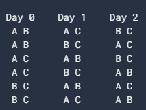
对于上图中的每一行,共有2^3 = 8种可能的方式将剩余的班次分配给护士(每天有两种选择)。 因此,可能分配的总数为108·6·8 = 5184。
eg2:一个常见的调度问题是作业车间,其中在多台机器上处理多个作业。每个作业都包含一系列任务,这些任务必须以给定的顺序执行,并且每个任务都必须在特定的计算机上进行处理。例如,工作可能是制造单个消费品,例如汽车。问题在于在机器上安排任务,以最大程度地减少安排时间(完成所有作业所花费的时间)。
作业车间问题有几个约束条件:在该作业的上一个任务完成之前,无法启动该作业的任务。一台机器一次只能执行一项任务。
任务一旦开始,就必须完成。
一个简单的车间问题示例,其中每个任务用一对数字(m,p)标记,其中m是必须在其上处理任务的机器的编号,p是任务的处理时间—所需的时间。 (作业和机器的编号从0开始。)
- job 0 = [(0, 3), (1, 2), (2, 2)]
- job 1 = [(0, 2), (2, 1), (1, 4)]
- job 2 = [(1, 4), (2, 3)]
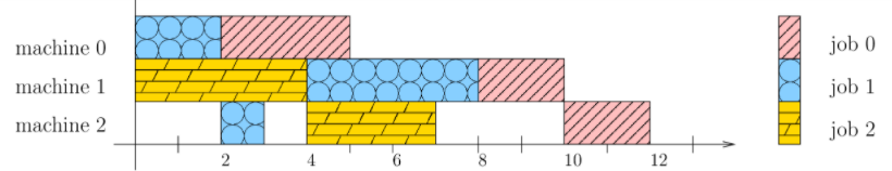
解决车间问题的方法是为每个任务分配一个开始时间,该时间要满足上述限制。
您可以检查每个作业的任务是否按问题给出的顺序按不重叠的时间间隔进行调度。该解决方案的长度为12,这是所有三个作业都第一次完成。这不是解决问题的最佳方法。
task(i,j)表示作业i的顺序中的第j个任务。例如,task(0,2)表示作业0的第二个任务,它对应于问题描述中的对(1、2)。
接下来,将ti,j定义为task(i,j)的开始时间。 ti,j是作业车间问题中的变量。寻找解决方案涉及确定满足问题要求的这些变量的值。
作业车间问题有两种约束:
优先约束-这些约束的条件是,对于同一作业中的任何两个连续任务,必须先完成第一个任务,然后才能启动第二个任务。例如,任务(0,2)和任务(0,3)是作业0的连续任务。由于任务(0,2)的处理时间为2,因此任务(0,3)的开始时间必须为在任务2的开始时间之后至少2个时间单位。(也许任务2正在粉刷一扇门,并且涂料需要干燥两个小时。)因此,您将获得以下约束: t0,2 + 2≤t0,3
没有重叠限制-这些限制是由于机器不能同时执行两个任务的限制而引起的。例如,task(0,2)和task(2,1)都在计算机1上处理。由于它们的处理时间分别为2和4,因此必须满足以下约束之一:
t0,2 + 2≤t2,1(如果任务(0,2)排在任务(2,1)之前)
要么
t2,1 + 4≤t0,2(如果task(2,1)排在task(0,2)之前)。
问题的目标
作业车间问题的目的是最大程度地减少制造时间:从作业的最早开始时间到最近结束时间的时间长度。
def eg_cp_JobshopSat():
    """Minimal jobshop problem."""
    # Create the model.
    model = cp_model.CpModel()

    jobs_data = [  # task = (machine_id, processing_time).
        [(0, 3), (1, 2), (2, 2)],  # Job0
        [(0, 2), (2, 1), (1, 4)],  # Job1
        [(1, 4), (2, 3)]  # Job2
    ]

    machines_count = 1 + max(task[0] for job in jobs_data for task in job)
    all_machines = range(machines_count)

    # Computes horizon dynamically as the sum of all durations.
    horizon = sum(task[1] for job in jobs_data for task in job)

    # Named tuple to store information about created variables.
    task_type = collections.namedtuple('task_type', 'start end interval')
    # Named tuple to manipulate solution information.
    assigned_task_type = collections.namedtuple('assigned_task_type',
                                                'start job index duration')

    # Creates job intervals and add to the corresponding machine lists.
    all_tasks = {}
    machine_to_intervals = collections.defaultdict(list)

    for job_id, job in enumerate(jobs_data):
        for task_id, task in enumerate(job):
            machine = task[0]
            duration = task[1]
            suffix = '_%i_%i' % (job_id, task_id)
            start_var = model.NewIntVar(0, horizon, 'start' + suffix)
            end_var = model.NewIntVar(0, horizon, 'end' + suffix)
            interval_var = model.NewIntervalVar(start_var, duration, end_var,
                                                'interval' + suffix)
            all_tasks[job_id, task_id] = task_type(
                start=start_var, end=end_var, interval=interval_var)
            machine_to_intervals[machine].append(interval_var)

    # Create and add disjunctive constraints.
    for machine in all_machines:
        model.AddNoOverlap(machine_to_intervals[machine])

    # Precedences inside a job.
    for job_id, job in enumerate(jobs_data):
        for task_id in range(len(job) - 1):
            model.Add(all_tasks[job_id, task_id +
                                1].start >= all_tasks[job_id, task_id].end)

    # Makespan objective.
    obj_var = model.NewIntVar(0, horizon, 'makespan')
    model.AddMaxEquality(obj_var, [
        all_tasks[job_id, len(job) - 1].end
        for job_id, job in enumerate(jobs_data)
    ])
    model.Minimize(obj_var)

    # Solve model.
    solver = cp_model.CpSolver()
    status = solver.Solve(model)

    if status == cp_model.OPTIMAL:
        # Create one list of assigned tasks per machine.
        assigned_jobs = collections.defaultdict(list)
        for job_id, job in enumerate(jobs_data):
            for task_id, task in enumerate(job):
                machine = task[0]
                assigned_jobs[machine].append(
                    assigned_task_type(
                        start=solver.Value(all_tasks[job_id, task_id].start),
                        job=job_id,
                        index=task_id,
                        duration=task[1]))

        # Create per machine output lines.
        output = ''
        for machine in all_machines:
            # Sort by starting time.
            assigned_jobs[machine].sort()
            sol_line_tasks = 'Machine ' + str(machine) + ': '
            sol_line = '           '

            for assigned_task in assigned_jobs[machine]:
                name = 'job_%i_%i' % (assigned_task.job, assigned_task.index)
                # Add spaces to output to align columns.
                sol_line_tasks += '%-10s' % name

                start = assigned_task.start
                duration = assigned_task.duration
                sol_tmp = '[%i,%i]' % (start, start + duration)
                # Add spaces to output to align columns.
                sol_line += '%-10s' % sol_tmp

            sol_line += '\n'
            sol_line_tasks += '\n'
            output += sol_line_tasks
            output += sol_line

        # Finally print the solution found.
        print('Optimal Schedule Length: %i' % solver.ObjectiveValue())
        print(output)
Optimal Schedule Length: 11
Machine 0: job_0_0 job_1_0
[0,3] [3,5]
Machine 1: job_2_0 job_0_1 job_1_2
[0,4] [4,6] [7,11]
Machine 2: job_1_1 job_0_2 job_2_1
[5,6] [6,8] [8,11]
N-皇后问题N-queens Problem
基于国际象棋游戏的组合问题来说明约束编程(CP)。 在国际象棋中,女王可以水平,垂直和对角线进攻。 N皇后问题问:如何将N个皇后放在NxN的棋盘上,使他们中没有两个互相攻击?在下面,您可以看到针对N = 4的N皇后问题的一种可能解决方案。

没有两个皇后在同一行,同一列或对角线上。
CP解算器的工作原理是系统地尝试对问题中的变量进行所有可能的值分配,以找到可行的解决方案。在4皇后问题中,求解器从最左列开始,并在每列中连续放置一个皇后,该位置不受任何先前放置的皇后的攻击。
约束编程搜索有两个关键元素:传播和回溯Propagation and backtracking
传播-求解器每次向变量分配值时,约束都会对未分配变量的可能值施加限制。这些限制会传播到将来的变量分配。例如,在4皇后问题中,求解器每次放置一个皇后,都无法在当前皇后所在的行和对角线上放置任何其他皇后。传播可以通过减少求解程序必须探索的变量值集来显着加快搜索速度。
回溯:当求解器由于约束而无法将值分配给下一个变量或找到解决方案时,就会发生回溯。无论哪种情况,求解器都会回溯到上一个阶段,并将该阶段的变量值更改为尚未尝试过的值。在4皇后示例中,这意味着将皇后移到当前列上的新正方形。
接下来,您将看到约束编程如何使用传播和回溯来解决4皇后问题。
假设求解器首先在左上角放置一个皇后开始。那是种假设。也许事实证明,左上角有一个皇后不存在任何解决方案。
在这种假设下,我们可以传播哪些约束?一个约束是一列中只能有一个皇后(下面的灰色Xs),另一个约束是禁止在同一对角线上有两个皇后,第三个约束禁止同一行上的皇后:

在一个可用的剩余方块上放置第二个女王。我们的解算器可能会决定将第二列中的第一个可用正方形放在它:

添加第二个皇后的限制条件

显然无法再放置剩下的2个皇后,因此这种方案就不成立,需要回溯。


from __future__ import print_function
import sys
from ortools.sat.python import cp_model


def main(board_size):
  model = cp_model.CpModel()
  # Creates the variables.
  # The array index is the column, and the value is the row.
  queens = [model.NewIntVar(0, board_size - 1, 'x%i' % i)
            for i in range(board_size)]
  # Creates the constraints.
  # The following sets the constraint that all queens are in different rows.
  model.AddAllDifferent(queens)

  # Note: all queens must be in different columns because the indices of queens are all different.

  # The following sets the constraint that no two queens can be on the same diagonal.
  for i in range(board_size):
    # Note: is not used in the inner loop.
    diag1 = []
    diag2 = []
    for j in range(board_size):
      # Create variable array for queens(j) + j.
      q1 = model.NewIntVar(0, 2 * board_size, 'diag1_%i' % i)
      diag1.append(q1)
      model.Add(q1 == queens[j] + j)
      # Create variable array for queens(j) - j.
      q2 = model.NewIntVar(-board_size, board_size, 'diag2_%i' % i)
      diag2.append(q2)
      model.Add(q2 == queens[j] - j)
    model.AddAllDifferent(diag1)
    model.AddAllDifferent(diag2)
  ### Solve model.
  solver = cp_model.CpSolver()
  solution_printer = SolutionPrinter(queens)
  status = solver.SearchForAllSolutions(model, solution_printer)
  print()
  print('Solutions found : %i' % solution_printer.SolutionCount())


class SolutionPrinter(cp_model.CpSolverSolutionCallback):
  """Print intermediate solutions."""

  def __init__(self, variables):
    cp_model.CpSolverSolutionCallback.__init__(self)
    self.__variables = variables
    self.__solution_count = 0

  def OnSolutionCallback(self):
    self.__solution_count += 1
    for v in self.__variables:
      print('%s = %i' % (v, self.Value(v)), end = ' ')
    print()

  def SolutionCount(self):
    return self.__solution_count


class DiagramPrinter(cp_model.CpSolverSolutionCallback):
  def __init__(self, variables):
    cp_model.CpSolverSolutionCallback.__init__(self)
    self.__variables = variables
    self.__solution_count = 0

  def OnSolutionCallback(self):
    self.__solution_count += 1

    for v in self.__variables:
      queen_col = int(self.Value(v))
      board_size = len(self.__variables)
      # Print row with queen.
      for j in range(board_size):
        if j == queen_col:
          # There is a queen in column j, row i.
          print("Q", end=" ")
        else:
          print("_", end=" ")
      print()
    print()

  def SolutionCount(self):
    return self.__solution_count


if __name__ == '__main__':
  # By default, solve the 8x8 problem.
  board_size = 8
  if len(sys.argv) > 1:
    board_size = int(sys.argv[1])
  main(board_size)
密码数学谜题Cryptarithmetic Puzzles
密码数学谜题是一种数学练习,其中某些数字的数字由字母(或符号)表示。每个字母表示唯一的数字。目标是查找数字,以便验证给定的数学方程:
例如CP+IS+FUN=TRUE,看的人看的是字母,字母到数字的过程实际上是23+74+968=1065
问题建模:十个字母中每个字母都必须是一个不同的数字,C 、I、F和T不能为零。组合第一个字母不可是0
"""Cryptarithmetic puzzle.

First attempt to solve equation CP + IS + FUN = TRUE
where each letter represents a unique digit.

This problem has 72 different solutions in base 10.
"""

from __future__ import print_function

from ortools.sat.python import cp_model


class VarArraySolutionPrinter(cp_model.CpSolverSolutionCallback):
    """Print intermediate solutions."""

    def __init__(self, variables):
        cp_model.CpSolverSolutionCallback.__init__(self)
        self.__variables = variables
        self.__solution_count = 0

    def on_solution_callback(self):
        self.__solution_count += 1
        for v in self.__variables:
            print('%s=%i' % (v, self.Value(v)), end=' ')
        print()

    def solution_count(self):
        return self.__solution_count


def CPIsFunSat():
    """Solve the CP+IS+FUN==TRUE cryptarithm."""
    # Constraint programming engine
    model = cp_model.CpModel()

    base = 10

    c = model.NewIntVar(1, base - 1, 'C')
    p = model.NewIntVar(0, base - 1, 'P')
    i = model.NewIntVar(1, base - 1, 'I')
    s = model.NewIntVar(0, base - 1, 'S')
    f = model.NewIntVar(1, base - 1, 'F')
    u = model.NewIntVar(0, base - 1, 'U')
    n = model.NewIntVar(0, base - 1, 'N')
    t = model.NewIntVar(1, base - 1, 'T')
    r = model.NewIntVar(0, base - 1, 'R')
    e = model.NewIntVar(0, base - 1, 'E')

    # We need to group variables in a list to use the constraint AllDifferent.
    letters = [c, p, i, s, f, u, n, t, r, e]

    # Verify that we have enough digits.
    assert base >= len(letters)

    # Define constraints.
    model.AddAllDifferent(letters)

    # CP + IS + FUN = TRUE
    model.Add(c * base + p + i * base + s + f * base * base + u * base +
              n == t * base * base * base + r * base * base + u * base + e)

    ### Solve model.
    solver = cp_model.CpSolver()
    solution_printer = VarArraySolutionPrinter(letters)
    status = solver.SearchForAllSolutions(model, solution_printer)

    print()
    print('Statistics')
    print('  - status          : %s' % solver.StatusName(status))
    print('  - conflicts       : %i' % solver.NumConflicts())
    print('  - branches        : %i' % solver.NumBranches())
    print('  - wall time       : %f s' % solver.WallTime())
    print('  - solutions found : %i' % solution_printer.solution_count())


if __name__ == '__main__':
    CPIsFunSat()
优化解题
目标使得 2x + 2y + 3z 最大,限制为:x, y, z integers
| x + 7⁄2 y + 3⁄2 z≤25 |
| 3x - 5y + 7z≤45 |
| 5x + 2y - 6z≤37 |
| x, y, z≥0 |
from __future__ import print_function
from ortools.sat.python import cp_model


def main():
  model = cp_model.CpModel()
  var_upper_bound = max(50, 45, 37)
  x = model.NewIntVar(0, var_upper_bound, 'x')
  y = model.NewIntVar(0, var_upper_bound, 'y')
  z = model.NewIntVar(0, var_upper_bound, 'z')

  model.Add(2*x + 7*y + 3*z <= 50)
  model.Add(3*x - 5*y + 7*z <= 45)
  model.Add(5*x + 2*y - 6*z <= 37)

  model.Maximize(2*x + 2*y + 3*z)

  solver = cp_model.CpSolver()
  status = solver.Solve(model)

  if status == cp_model.OPTIMAL:
    print('Maximum of objective function: %i' % solver.ObjectiveValue())
    print()
    print('x value: ', solver.Value(x))
    print('y value: ', solver.Value(y))
    print('z value: ', solver.Value(z))


if __name__ == '__main__':
  main()
如果程序运行时间很长,我们建议为解算器设置时间限制,以确保程序将在合理的时间长度内终止。下面的示例演示了如何为解算器设置 10 秒的限制。
# Sets a time limit of 10 seconds.
solver.parameters.max_time_in_seconds = 10.0
作为设置时间限制的替代方法,可以使解算器在找到指定数量的解决方案后终止。例如找到5个方案就停止
class VarArraySolutionPrinterWithLimit(cp_model.CpSolverSolutionCallback):
    """Print intermediate solutions."""

    def __init__(self, variables, limit):
        cp_model.CpSolverSolutionCallback.__init__(self)
        self.__variables = variables
        self.__solution_count = 0
        self.__solution_limit = limit

    def on_solution_callback(self):
        self.__solution_count += 1
        for v in self.__variables:
            print('%s=%i' % (v, self.Value(v)), end=' ')
        print()
        if self.__solution_count >= self.__solution_limit:
            print('Stop search after %i solutions' % self.__solution_limit)
            self.StopSearch()

    def solution_count(self):
        return self.__solution_count

solution_printer = VarArraySolutionPrinterWithLimit([x, y, z], 5)


 3895
3895


 被折叠的 条评论
为什么被折叠?
被折叠的 条评论
为什么被折叠?
 到【灌水乐园】发言


