


目录
一.引言
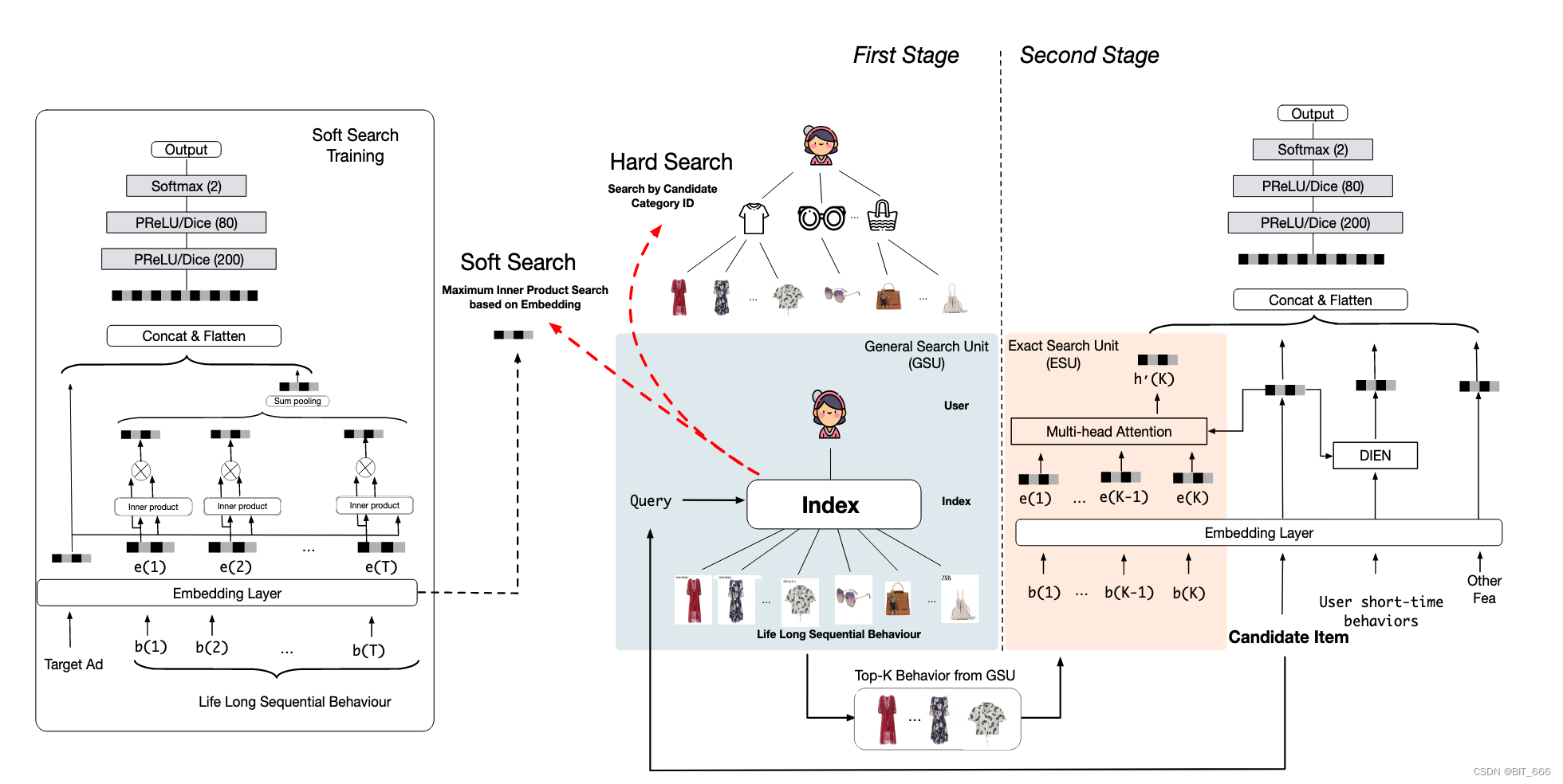
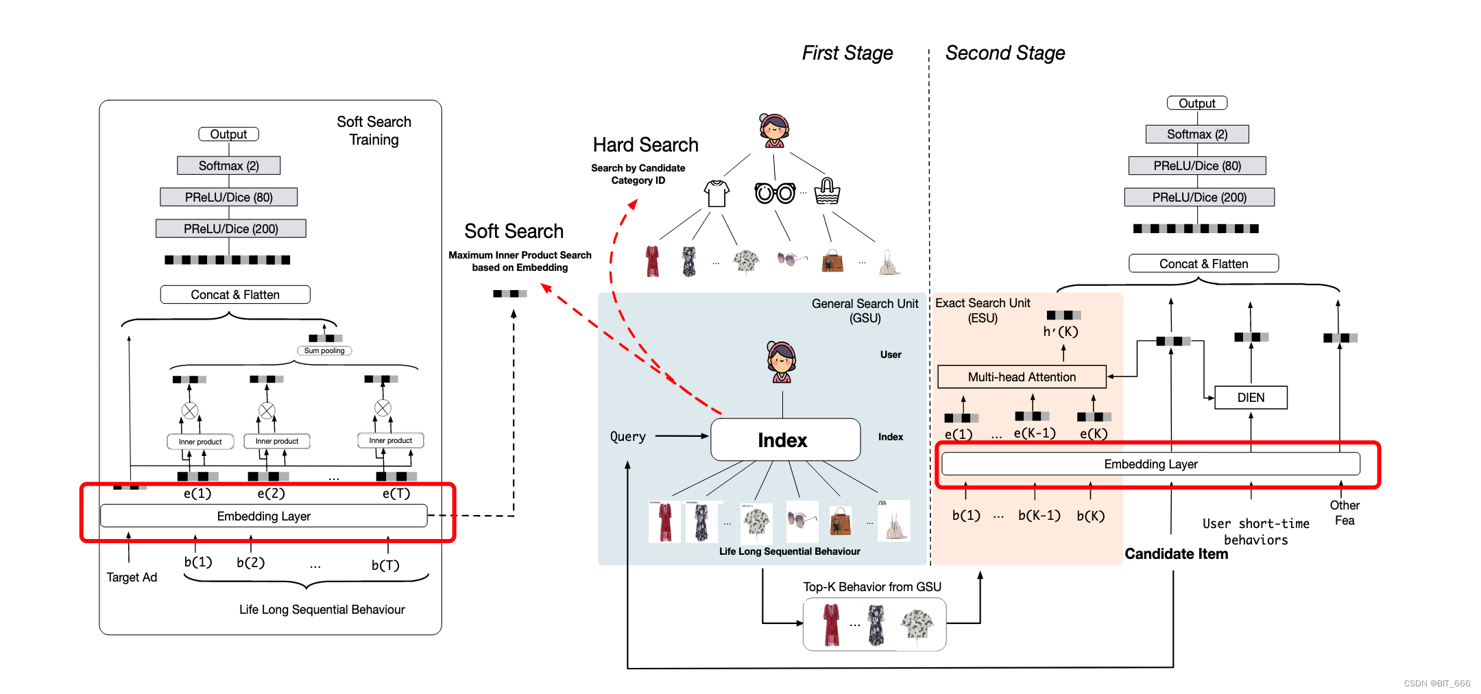
SIM 引入两阶段兴趣搜索,通过 GSU 通用搜索单元从长序列中快速匹配与 Item 相关的用户长期兴趣生成相关子用户序列 SBS,并通过 ESU 模拟候选 Item 与 SBS 之间的精确关系。其中 GSU 模块一般有 Soft Search 和 Hard Search 两种方法,下面基于 keras 简单实现下 Soft Search 软搜索并根据内积生成 SBS。
二.GSU 结构分析
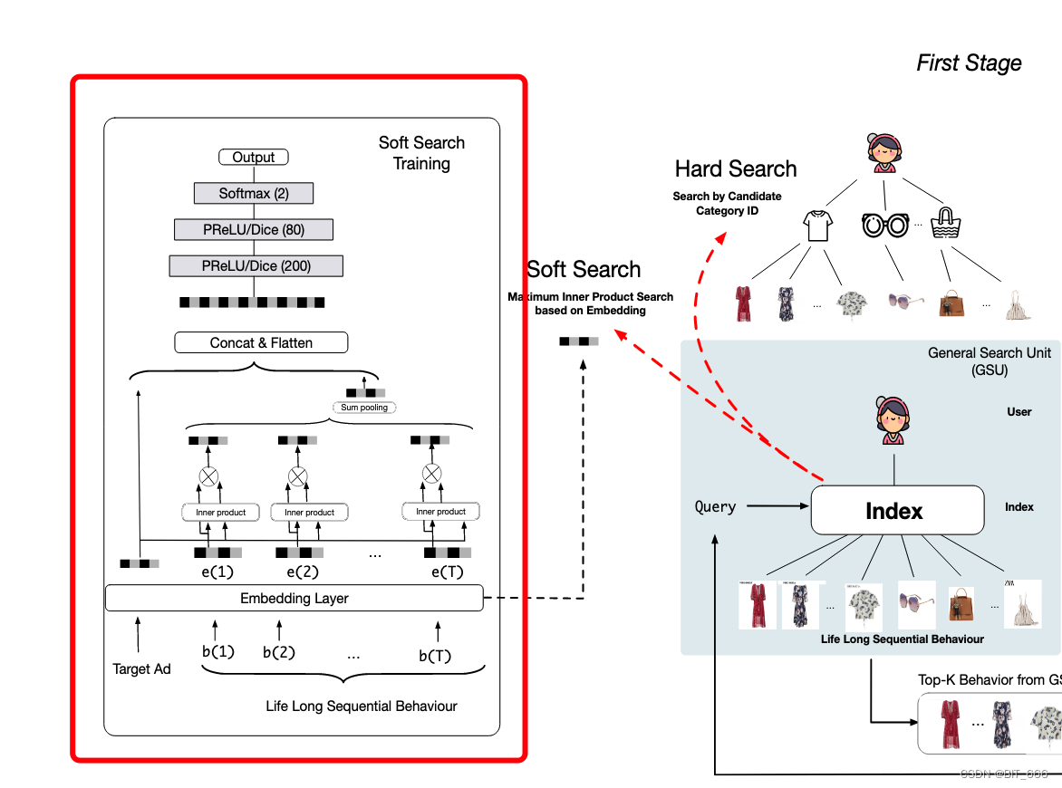
GSU - General search Unit 指的是 SIM 模型的通用搜索模块单元,关于 SIM 的具体论文细节大家可以参考:SIM 论文笔记,本文主要基于 keras 实现简单 GSU 的 Soft Search,其模块如下图红框所示。
1.Input Layer 输入层
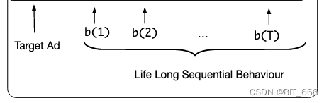
输入层包括 Target Ad 目标广告以及用户对应的长期序列行为,论文中认为 <= 14 天的行为为短期行为,> 14 天发生的行为为长期行为,并构造了 d-category metrics 进行了模型评估。
2.Embedding Layer 嵌入层
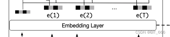
将上述 Ad-id 以及 b(i) 对应的 good-id lookup 获取对应 Embedding 嵌入。
Tips:
论文中认为用户长期行为与短期行为的分布不同,所以长期行为的 Embedding Layer 和短期行为对应的 Embedding Layer 并不共享,如下图红框所示,虽然 id 集合相同,但是 Embedding Layer 是分开构建的。
3.Pooling Layer 池化层
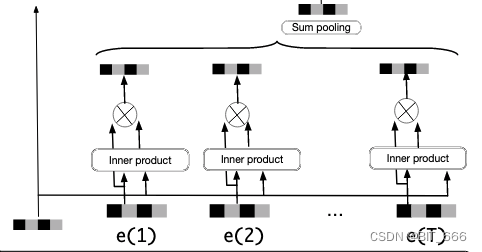
这里用长序列个每个 good Embedding 向量与 target Ad 的 Embedding 向量内积得到权重 Wi,然后 Wi 元素乘对应 good Embedding 做加权的 Sum Pooling,当然大家也可以尝试例如 Mean Pooling 这样的池化方式。
4.MLP 深层网络
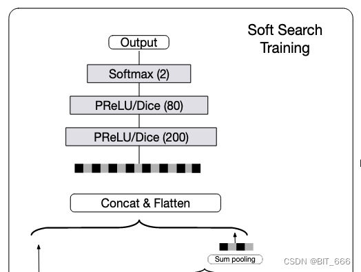
最后一步遵循传统的 MLP 范式,将 Target Ad 的 Embedding 与长序列 Sum Pooling 得到的 Embedding 一起 Concat 传给 MLP 层,其层数分别为 200、80、2,与 DIN 类似,采用了 PRelu / Dice 激活函数,最后的 softmax 输出结果。
5.Soft Search 软搜索
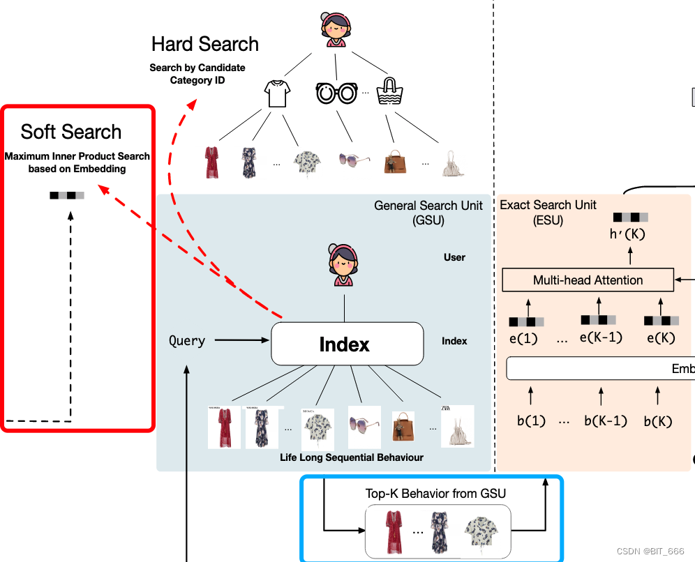
Soft Search 通过 Maximum Inner Product 最大内积搜索与 Query 相近的 Top-K Behavior In GSU,其中 DIN、DIEN 使用的序列长度一般为 150,这里论文 K 选择 150-200 的范围。
三.GSU 结构实现
全部依赖如下,其中 Dice 激活可以参考:DIN 实现 By Keras。
import numpy as np
import tensorflow as tf
from tensorflow.keras import Model
from tensorflow.keras.layers import Dense, Layer
from tensorflow.python.keras import Input
from tensorflow.python.ops.init_ops import TruncatedNormal
from DIN import Dice
from tensorflow.keras import backend as K
import heapq
1.Init 初始化
class GSULayer(Layer):

    def __init__(self, N=10000, embedding_dim=8, pooling_mode='sum', **kwargs):

        # 序列相关
        self.N = N
        self.embedding_dim = embedding_dim
        self.pooling_mode = pooling_mode
        self.T = None

        # 参数矩阵
        self.kernel = None
        self.weight_normalization = True

        self.DNN_3 = None
        self.DNN_2 = None
        self.DNN_1 = None

        super(GSULayer, self).__init__(**kwargs)
根据上面分析的 GSU Soft Search 模块,初始化定义如下变量:
N - 商品库大小
embedding_dim - 嵌入向量维度
pooling_mode - [sum、mean] 求和与求平均
T - 用户序列长度
kernel - Embedding Layer
weight_normalization - 权重是否归一化
DNN_I - MLP 对应的 200、80、2 的隐层
2.Build 构建
    def build(self, input_shape):
        # 获取序列长度
        history_shape, candidate_shape = input_shape
        self.T = history_shape[1]

        # N x embedding_dim 的参数矩阵
        self.kernel = self.add_weight(name='kernel',
                                      shape=(self.N, self.embedding_dim),
                                      initializer=TruncatedNormal,
                                      trainable=True)

        # 构建 DNN
        self.DNN_1 = Dense(200, activation=Dice())
        self.DNN_2 = Dense(80, activation=Dice())
        self.DNN_3 = Dense(1, activation='sigmoid')

        super(GSULayer, self).build(input_shape)
build 函数主要实现上述 init 变量的初始化,这里模型采用多输入模式,所以 history_shape 和 candidate_shape 是分开的,通过 history_shape 可以解析得到 T 序列长度。向量层大小为 N x embedding_dim,Dense 层的最后一层与原文略有不同,文章采用 Dense(2) + Softmax 的方式,这里采用 Dense(1) + Sigmoid 的方式。
3.call 调用
• 获取 Item、History 嵌入
    # 1.获取历史行为、候选集 Embedding 5x100x8, 5x1x8
    _history, _candidate = inputs  # [None, 10] [None, 1]
    # [None, T] => [None, T, embedding_dim]
    history_emd = tf.nn.embedding_lookup(self.kernel, _history)

    # [None, 1] => [None, 1, embedding_dim] => [None, T, embedding_dim]
    candidate_emb = tf.nn.embedding_lookup(self.kernel, _candidate)
    repeat_candidate_emb = K.repeat_elements(candidate_emb, self.T, axis=1)
直接 lookup 得到对应 Embedding 嵌入。
• Item 与 Good 计算内积
    # 内积计算权重
    dot_weights = tf.multiply(history_emd, repeat_candidate_emb)
    dot_weights = tf.reduce_sum(dot_weights, axis=2)

    if self.weight_normalization:
        dot_weights = tf.nn.softmax(dot_weights)
计算内积获得每个 Good 对应的权重 W,并根据参数决定是否归一化。
• 加权求和
    # 对 History 加权
    dot_weights = tf.reshape(dot_weights, [-1, self.T, 1])
    add_weights = history_emd * dot_weights

    # Sum Pooling
    if self.pooling_mode == "sum":
        pooling_output = tf.reduce_sum(add_weights, axis=1)
    else:
        pooling_output = tf.reduce_mean(add_weights, axis=1)
加权相乘后进行 pooling 操作,论文中采用 sum-pooling 求和方式池化。
• Concat && MLP
    # Concat
    candidate_emb = tf.reshape(candidate_emb, shape=(-1, self.embedding_dim))
    concat = tf.concat([candidate_emb, pooling_output], axis=-1)

    _output = self.DNN_1(concat)
    _output = self.DNN_2(_output)
    _output = self.DNN_3(_output)
Concat + MLP 的经典推荐模型范式,这里 DNN 也可以采用三层嵌套的写法。
4.GSU Layer 完整代码
class GSULayer(Layer):

    def __init__(self, N=10000, embedding_dim=8, pooling_mode='sum', **kwargs):

        # 序列相关
        self.N = N
        self.embedding_dim = embedding_dim
        self.pooling_mode = pooling_mode
        self.T = None

        # 参数矩阵
        self.kernel = None
        self.weight_normalization = True

        self.DNN_3 = None
        self.DNN_2 = None
        self.DNN_1 = None

        super(GSULayer, self).__init__(**kwargs)

    def build(self, input_shape):
        # 获取序列长度
        history_shape, candidate_shape = input_shape
        self.T = history_shape[1]

        # N x embedding_dim 的参数矩阵
        self.kernel = self.add_weight(name='kernel',
                                      shape=(self.N, self.embedding_dim),
                                      initializer=TruncatedNormal,
                                      trainable=True)

        # 构建 DNN
        self.DNN_1 = Dense(200, activation=Dice())
        self.DNN_2 = Dense(80, activation=Dice())
        self.DNN_3 = Dense(1, activation='sigmoid')

        super(GSULayer, self).build(input_shape)

    def call(self, inputs, **kwargs):
        # 1.获取历史行为、候选集 Embedding 5x100x8, 5x1x8
        _history, _candidate = inputs  # [None, 10] [None, 1]
        # [None, T] => [None, T, embedding_dim]
        history_emd = tf.nn.embedding_lookup(self.kernel, _history)

        # [None, 1] => [None, 1, embedding_dim] => [None, T, embedding_dim]
        candidate_emb = tf.nn.embedding_lookup(self.kernel, _candidate)
        repeat_candidate_emb = K.repeat_elements(candidate_emb, self.T, axis=1)

        # 内积计算权重
        dot_weights = tf.multiply(history_emd, repeat_candidate_emb)
        dot_weights = tf.reduce_sum(dot_weights, axis=2)

        if self.weight_normalization:
            dot_weights = tf.nn.softmax(dot_weights)

        # 对 History 加权
        dot_weights = tf.reshape(dot_weights, [-1, self.T, 1])
        add_weights = history_emd * dot_weights

        # Sum Pooling
        if self.pooling_mode == "sum":
            pooling_output = tf.reduce_sum(add_weights, axis=1)
        else:
            pooling_output = tf.reduce_mean(add_weights, axis=1)

        # Concat
        candidate_emb = tf.reshape(candidate_emb, shape=(-1, self.embedding_dim))
        concat = tf.concat([candidate_emb, pooling_output], axis=-1)

        _output = self.DNN_1(concat)
        _output = self.DNN_2(_output)
        _output = self.DNN_3(_output)

        return _output

    def compute_output_shape(self, input_shape):
        return input_shape[0][0], 1
四.GSU 模型训练
下面基于 GSU Layer 与模拟输入进行 Soft Search。
1.Input Layer
    # 批次大小、序列长度、商品类目
    batch_size, T, N = 5, 10000, 1000000

    # 多输入模型
    historyForGSU = Input(shape=(T,), dtype='int32', name='history')
    candidateForGSU = Input(shape=(1,), dtype='int32', name='candidate')
历史行为序列长度为 T,候选集长度为 1,论文中候选集的长度可以达到 54000,是先前 MIMN 记忆网络的 54x。
2.GSU Layer
    # Sum Pooling
    GSU = GSULayer(N=N, embedding_dim=8, pooling_mode='sum', name="GSU")
    outputByGSU = GSU([historyForGSU, candidateForGSU])
基础的多输入模型,采用 sum pooling。
3.GSU Model
# 交叉熵二分类模型
GSU_model = Model(inputs=[historyForGSU, candidateForGSU], outputs=[outputByGSU])
GSU_model.compile(optimizer='rmsprop',
loss={'GSU': 'binary_crossentropy'},
loss_weights={'GSU': 1})
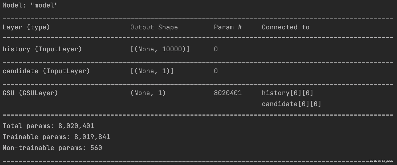
GSU_model.summary()添加损失函数与优化器,模型 summary 如下,论文中嵌入维度为 4,这里嵌入维度为 8,可以看到随着商品库数量的增加,模型参数的数量也很可观。
4.模拟序列样本生成
def genSamplesWithLabel(batch_size=5, T=10, N=1000, seed=0):
np.random.seed(seed)
# 用户历史序列
user_history = np.random.randint(0, N, size=(batch_size, T))
# 候选 Item
user_candidate = np.random.randint(0, N, size=(batch_size, 1))
# Labels
sample_labels = np.random.randint(0, 2, size=batch_size)
return user_history, user_candidate, sample_labels
# 用户历史行为序列 && 候选商品 ID
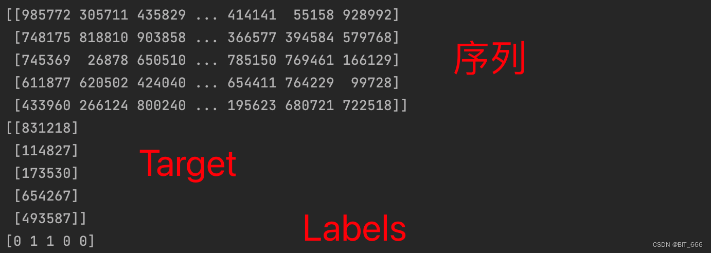
history, candidate, labels = genSamplesWithLabel(batch_size, T, N)样本样例如下:
5.模型 Fit
# GSU 长期序列行为训练
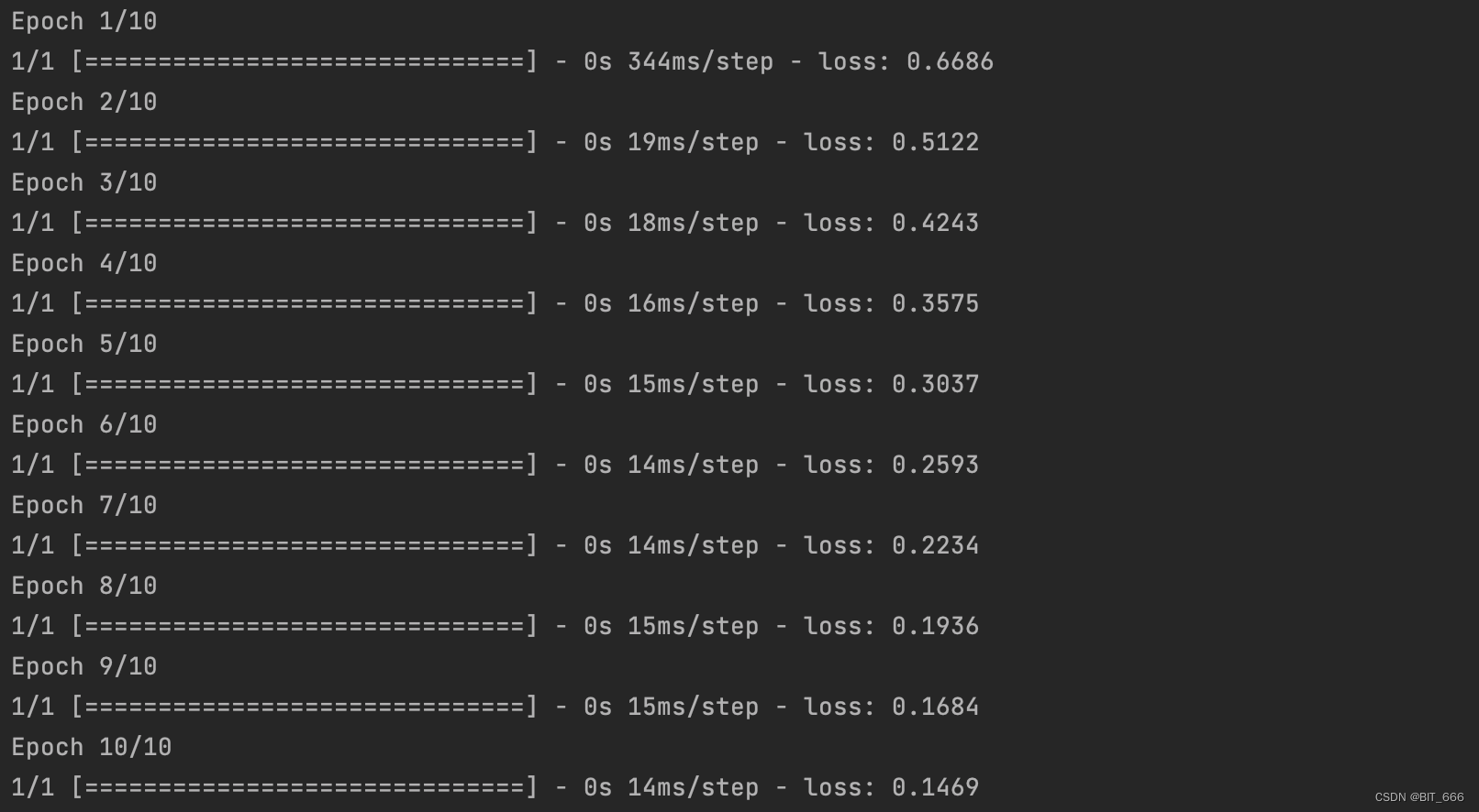
GSU_model.fit([history, candidate], labels, epochs=10, batch_size=128)示例样本,fit 只是走通流程,metric 不做参考:
五.Soft Search 软搜索
为了进一步加快万长度用户行为 Top-K 搜索速度,基于嵌入向量 E,论文中采用亚线性时间最大内积搜索方法 ALSH,搜索与目标项相关的 Top-K 行为。之前论文中还介绍过局部敏感 Hash 分桶的快速缓存搜索方法,这里示例使用最大堆 Heap 实现简易 Maximum Inner Product 的 Top-K 方法。
1.获取 Embedding 参数
kernel = np.array(GSU_model.get_layer("GSU").get_weights()[0])kernel 即为商品的嵌入层,其维度为 N x embedding_dim,本例中 Kernel Size = (1000000, 8)。
2.Soft Search
通过 heapq.nlargers 实现 Top-K Good 的排序,然后基于 Top-K Good 的 Index 索引构建 SBS 用户长期行为子序列,送到后面的 ESU 通过 Attention 机制进行精确搜索。
class SoftSearch:

    def __init__(self, _kernel, _K):
        self.kernel = _kernel
        self.K = _K
        print("Kernel Size:", kernel.shape)

    def genTopK(self, good_history, target):

        _topKGoods = []
        _topKScores = []

        for sample in zip(good_history, target):
            score = []
            cur_seq, cur_tar = sample
            cur_tar_emd = np.squeeze(kernel[cur_tar])
            for seq in cur_seq:
                score.append(np.dot(kernel[seq], cur_tar_emd))
            # 获取下标
            topKIndex = heapq.nlargest(self.K, range(len(score)), score.__getitem__)
            # 获取数值
            topKScore = heapq.nlargest(self.K, score)

            _topKGoods.append(topKIndex)
            _topKScores.append(topKScore)

        return _topKGoods, _topKScores
3.Soft Search 取 Top-K
论文中 Top-K 的 K 取 200 送入 GSU,这里示例取 10 跑通 Demo。
K = 10
search = SoftSearch(kernel, K)
topKGoods, topKScores = search.genTopK(history, candidate)
for SBS, Score in zip(topKGoods, topKScores):
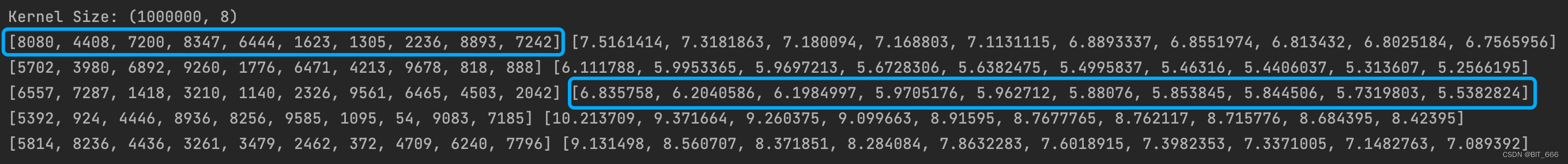
print(SBS, Score)其中 SBS 的长度为 K,后面的 Scores 是内积后排序的依据,这里是从大到小取 Top。
六.总结
至此,简易的 GUS with Soft Search 就实现了,论文中由于软搜索与硬搜索得到的 SBS 序列相近且大部分为对应 Item 的同 Cate 类型商品,在权衡性能收益与资源消耗后,阿里巴巴选择使用 Hard Search 即 KKV 的形式进行 GSU 的通用搜索,但是这不妨碍 Soft Search 可以作为一种 Embedding 预训练的方式挖掘长期商品对应的向量。
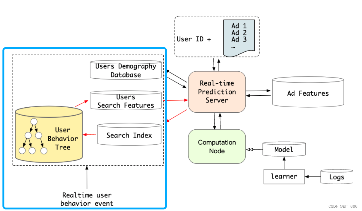
工程上阿里巴巴采用 Tree 的形式构造 KKV 存储结构。


 被折叠的 条评论
为什么被折叠?
被折叠的 条评论
为什么被折叠?
 到【灌水乐园】发言


