【完结】cyのLastDance - Chapter2（20241030~20241117）

序言

首马备赛篇——伤后半年的第二次挑战，目标依然是破三。

昨日赛后，明显状态好转，之前还是心理作用大一些。默认自己不行，就真的不行了。

尽管事难如愿，但开始自我怀疑的时候，就已经失败了。

常想一二，不思八九。

老家伙们该退场了。

---

---

20241030

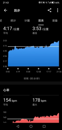
• 晚上九点下去摇了会儿，一共8K多，把月跑量补到180K，月均配4’10"，明后台风登陆，这个月大概率是凑不到200K了。

• 逮到DGL，她是真的马不停蹄，练得太狠了，昨天参加800米、3000米、4×400米三项，今天又是5组800米间歇，我给她带了一组，前后还有一共3K多的慢跑，真佩服年轻人的精力。

• PS：这次校运会照片真的不少，有5000多张，学校难得做了回人事。

DQN进阶之Nature DQN：

在NIPS2013中，DQN的目标Q值计算公式：

$$y_j=\{\begin{array}{rlrl}& R_j& & isen{d}_{j}istrue\\ & R_j+\gamma \underset{a^{\prime }}{\max }Q(\varphi (S_j^{\prime }),A_j^{\prime },w)& & isen{d}_{j}isfalse\end{array}$$

这里目标Q值的计算使用到了当前要训练的Q网络参数来计算$Q(\varphi (S_j^{\prime }),A_j^{\prime },w)$，而实际上，我们又希望通过$y_j$来后续更新Q网络参数，这样两者循环依赖，迭代起来相关性太强，不利于算法收敛。因此，一个改进版的Nature DQN尝试用两个Q网络来减少目标Q值计算和要更新Q网络参数之间的依赖关系。

Nature DQN使用了两个Q网络，一个当前Q网络
$Q$用来选择动作，更新模型参数，另一个目标Q网络$Q^{\prime }$用于计算目标Q值。目标Q网络的网络参数不需要迭代更新，而是每隔一段时间从当前Q网络$Q$，复制过来，即延时更新，这样可以减少目标Q值和当前的Q值相关性。

要注意的是，两个Q网络的结构是一模一样的。这样才可以复制网络参数。

首先是Q网络，上一篇的DQN是一个三层的神经网络，而这里我们有两个一样的三层神经网络，一个是当前Q网络，一个是目标Q网络，网络的定义部分如下：代码

def create_Q_network(self):
    # input layer
    self.state_input = tf.placeholder("float", [None, self.state_dim])
    # network weights
    with tf.variable_scope('current_net'):
        W1 = self.weight_variable([self.state_dim,20])
        b1 = self.bias_variable([20])
        W2 = self.weight_variable([20,self.action_dim])
        b2 = self.bias_variable([self.action_dim])

        # hidden layers
        h_layer = tf.nn.relu(tf.matmul(self.state_input,W1) + b1)
        # Q Value layer
        self.Q_value = tf.matmul(h_layer,W2) + b2

    with tf.variable_scope('target_net'):
        W1t = self.weight_variable([self.state_dim,20])
        b1t = self.bias_variable([20])
        W2t = self.weight_variable([20,self.action_dim])
        b2t = self.bias_variable([self.action_dim])

        # hidden layers
        h_layer_t = tf.nn.relu(tf.matmul(self.state_input,W1t) + b1t)
        # Q Value layer
        self.target_Q_value = tf.matmul(h_layer,W2t) + b2t

对于定期将目标Q网络的参数更新的代码如下面两部分：

    t_params = tf.get_collection(tf.GraphKeys.GLOBAL_VARIABLES, scope='target_net')
    e_params = tf.get_collection(tf.GraphKeys.GLOBAL_VARIABLES, scope='current_net')

    with tf.variable_scope('soft_replacement'):
        self.target_replace_op = [tf.assign(t, e) for t, e in zip(t_params, e_params)]

  def update_target_q_network(self, episode):
    # update target Q netowrk
    if episode % REPLACE_TARGET_FREQ == 0:
        self.session.run(self.target_replace_op)
        #print('episode '+str(episode) +', target Q network params replaced!')

此外，注意下我们计算目标Q值的部分，这里使用的目标Q网络的参数，而不是当前Q网络的参数：

    # Step 2: calculate y
    y_batch = []
    Q_value_batch = self.target_Q_value.eval(feed_dict={self.state_input:next_state_batch})
    for i in range(0,BATCH_SIZE):
      done = minibatch[i][4]
      if done:
        y_batch.append(reward_batch[i])
      else :
        y_batch.append(reward_batch[i] + GAMMA * np.max(Q_value_batch[i]))

---

20241031

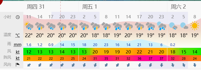
• 南马号码簿公布，不幸分在F区，SABC第一枪7:30出发，DEFG第二枪7:45出发，虽然两枪相隔很长时间，但一共24000人实在是太多了，AK在A区，肯定是带不了我，想破三只能靠自己。

• 看windy上的预报从今晚开始，暴雨一直要下到明晚，于是晚上吃完饭就润回去了，食物饮水都备好，已经做好明天宅一天的准备。还没在上海经历过台风天，今年自从魔都结界破了之后，这已经是第三回台风来袭，前两回都是躲过了，这次不知道会是个啥子情况，emmm
  

解决git拉取文件字符不合法问题：如有些文件包含星号，在

忽略转义字符

git config --global core.protectNTFS false

禁用换行符转换

git config --global core.autocrlf false

中文文件名，乱码问题。设为false的话，就不会对0x80以上的字符进行quot

git config --global core.quotepath false

DQN进阶之DDQN

在DDQN之前，基本上所有的目标Q值都是通过贪婪法直接得到的，无论是Q-Learning，DQN(NIPS 2013)还是Nature DQN，都是如此。

使用max虽然可以快速让Q值向可能的优化目标靠拢，但是很容易过犹不及，导致过度估计(Over Estimation)，所谓过度估计就是最终我们得到的算法模型有很大的偏差(bias)。为了解决这个问题， DDQN通过解耦目标Q值动作的选择和目标Q值的计算这两步，来达到消除过度估计的问题。

DDQN和Nature DQN一样，也有一样的两个Q网络结构。在Nature DQN的基础上，通过解耦目标Q值动作的选择和目标Q值的计算这两步，来消除过度估计的问题。

在Nature DQN中，目标Q值计算公式为：

$$y_j=R_j+\gamma \underset{a^{\prime }}{\max }{Q}^{\prime }(\varphi (S_j^{\prime }),A_j^{\prime },w^{\prime })$$

在DDQN中，不再是在目标Q网络中找各个动作的最大Q值，而是先在当前Q网络中找最大Q值对应的动作：

$$a^{\max }(S_j^{\prime },w)=\arg \underset{a^{\prime }}{\max }Q(\varphi (S_j^{\prime }),a,w)$$

然后利用选出来的$a^{\max }(S_j^{\prime },w)$在目标网络中计算目标Q值，即：

$$y_j=R_j+\gamma \underset{a^{\prime }}{\max }{Q}^{\prime }(\varphi (S_j^{\prime }),\arg \underset{a^{\prime }}{\max }Q(\varphi (S_j^{\prime }),a,w),w^{\prime })$$

其余与Nature DQN完全相同

代码只有一个地方不一样，就是计算目标Q值的时候，如下：

# Step 2: calculate y
y_batch = []
current_Q_batch = self.Q_value.eval(feed_dict={self.state_input: next_state_batch})
max_action_next = np.argmax(current_Q_batch, axis=1)
target_Q_batch = self.target_Q_value.eval(feed_dict={self.state_input: next_state_batch})

for i in range(0,BATCH_SIZE):
  done = minibatch[i][4]
  if done:
    y_batch.append(reward_batch[i])
  else :
    target_Q_value = target_Q_batch[i, max_action_next[i]]
    y_batch.append(reward_batch[i] + GAMMA * target_Q_value)

而之前的Nature DQN这里的目标Q值计算是如下这样的：

# Step 2: calculate y
y_batch = []
Q_value_batch = self.target_Q_value.eval(feed_dict={self.state_input:next_state_batch})
for i in range(0,BATCH_SIZE):
  done = minibatch[i][4]
  if done:
    y_batch.append(reward_batch[i])
  else :
    y_batch.append(reward_batch[i] + GAMMA * np.max(Q_value_batch[i]))

---

20241101

• 小风小雨，完全比不上上次的破坏力，还指望把田径场刚修好的围栏再吹倒，到晚上已经基本复原。

• 跑休两日，明日准备起早30K，本周末也是柴古越野和市运会，会是个好天气。

Prioritized Replay DQN

在Prioritized Replay DQN之前，在采样的时候，我们是一视同仁，在经验回放池里面的所有的样本都有相同的被采样到的概率。

注意到在经验回放池里面的不同的样本由于TD误差的不同，对我们反向传播的作用是不一样的。TD误差越大，那么对我们反向传播的作用越大。而TD误差小的样本，由于TD误差小，对反向梯度的计算影响不大。在Q网络中，TD误差就是目标Q网络计算的目标Q值和当前Q网络计算的Q值之间的差距。这样如果TD误差的绝对值$|\delta |$较大的样本更容易被采样，则我们的算法会比较容易收敛。下面我们看看Prioritized Replay DQN的算法思路。

Prioritized Replay DQN根据每个样本的TD误差绝对值$|\delta |$，给定该样本的优先级正比于$|\delta |$将这个优先级的值存入经验回放池。回忆下之前的DQN算法，我们仅仅只保存和环境交互得到的样本状态，动作，奖励等数据，没有优先级这个说法。

由于引入了经验回放的优先级，那么Prioritized Replay DQN的经验回放池和之前的其他DQN算法的经验回放池就不一样了。因为这个优先级大小会影响它被采样的概率。在实际使用中，我们通常使用SumTree这样的二叉树结构来做我们的带优先级的经验回放池样本的存储。

具体的SumTree树结构如下图：

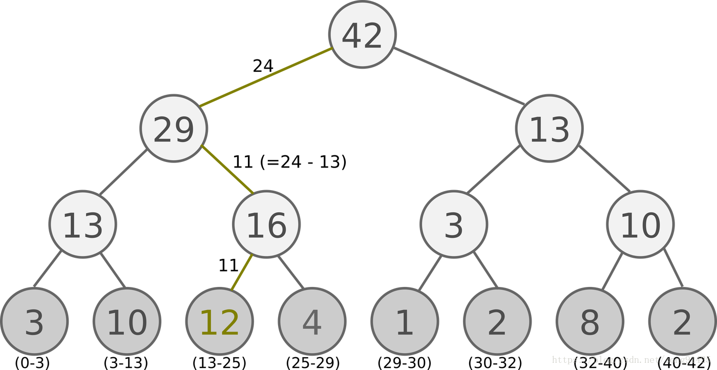
所有的经验回放样本只保存在最下面的叶子节点上面，一个节点一个样本。内部节点不保存样本数据。而叶子节点除了保存数据以外，还要保存该样本的优先级，就是图中的显示的数字。对于内部节点每个节点只保存自己的儿子节点的优先级值之和，如图中内部节点上显示的数字。

这样保存有什么好处呢？主要是方便采样。以上面的树结构为例，根节点是42，如果要采样一个样本，那么我们可以在[0,42]之间做均匀采样，采样到哪个区间，就是哪个样本。比如我们采样到了26， 在（25-29）这个区间，那么就是第四个叶子节点被采样到。而注意到第三个叶子节点优先级最高，是12，它的区间13-25也是最长的，会比其他节点更容易被采样到。

如果要采样两个样本，我们可以在[0,21],[21,42]两个区间做均匀采样，方法和上面采样一个样本类似。

def sample(self, n):
        b_idx, b_memory, ISWeights = np.empty((n,), dtype=np.int32), np.empty((n, self.tree.data[0].size)), np.empty((n, 1))
        pri_seg = self.tree.total_p / n       # priority segment
        self.beta = np.min([1., self.beta + self.beta_increment_per_sampling])  # max = 1

        min_prob = np.min(self.tree.tree[-self.tree.capacity:]) / self.tree.total_p     # for later calculate ISweight
        if min_prob == 0:
            min_prob = 0.00001
        for i in range(n):
            a, b = pri_seg * i, pri_seg * (i + 1)
            v = np.random.uniform(a, b)
            idx, p, data = self.tree.get_leaf(v)
            prob = p / self.tree.total_p
            ISWeights[i, 0] = np.power(prob/min_prob, -self.beta)
            b_idx[i], b_memory[i, :] = idx, data
        return b_idx, b_memory, ISWeights

除了采样部分，要注意的就是当梯度更新完毕后，我们要去更新SumTree的权重，代码如下，注意叶子节点的权重更新后，要向上回溯，更新所有祖先节点的权重。

def get_leaf(self, v):
        """
        Tree structure and array storage:
        Tree index:
             0         -> storing priority sum
            / \
          1     2
         / \   / \
        3   4 5   6    -> storing priority for transitions
        Array type for storing:
        [0,1,2,3,4,5,6]
        """
        parent_idx = 0
        while True:     # the while loop is faster than the method in the reference code
            cl_idx = 2 * parent_idx + 1         # this leaf's left and right kids
            cr_idx = cl_idx + 1
            if cl_idx >= len(self.tree):        # reach bottom, end search
                leaf_idx = parent_idx
                break
            else:       # downward search, always search for a higher priority node
                if v <= self.tree[cl_idx]:
                    parent_idx = cl_idx
                else:
                    v -= self.tree[cl_idx]
                    parent_idx = cr_idx

        data_idx = leaf_idx - self.capacity + 1
        return leaf_idx, self.tree[leaf_idx], self.data[data_idx]

Prioritized Replay DQN和DDQN相比，收敛速度有了很大的提高，避免冗余的迭代。

---

20241102

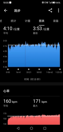
• 30K挑战失败，10K多有点岔气，均配407，停下来休息了会儿，接着又跑了2K@404还是不太行，感觉肯定坚持不到30K，太阳也有点大，索性还是不折磨自己了。

• 节奏尚可，感觉410的配肯定是能坚持很久，但是也明显感觉得到目前状态不如三月，全程心率几乎都在170左右，破三的信心依然不是很足。
  

• 下午白辉龙带YY跑6000米+200米×20组间歇，配速3分整，间歇200米慢跑，量非常大，实际上200米都跑到了35秒以内，最后一组30秒，他校运会失利后还是很受刺激的，下定决心要狠狠练，上限注定很高。

• 战报：

  • AK柴古55K组6小时59分完赛，虽然不如去年的表现，但排名倒是上升了（去年6小时34分，排名49，今年47），喜提红马甲。
    

  • 市运会5000米，小崔17分55秒，中途紧跟隔壁车浩然，虽然最后被拉爆了（车神16分38秒，发挥真的稳）；AX18分33秒，AX又数错圈，少跑一圈停下来五六秒才反应过来，估计是被小崔传染了。两人表现皆不如校运会，不过也是正常发挥，没有人能一直PB的。

  • 其余未知，不知道DGL的1500米和3000米怎么样，可能是明天，反正是没听到消息，之前听说可能会放掉保接力，不过我觉得她练这么狠肯定还是希望在个人项目上跑个好成绩。

对偶DQN

在Prioritized Replay DQN中，优化经验回放池按权重采样来优化算法。在Dueling DQN中，则通过优化神经网络的结构来优化算法。

Dueling DQN考虑将Q网络分成两部分，第一部分是仅与状态$S$相关，与动作$A$无关，这部分叫作价值函数，记作$V(S,w,\alpha )$，第二部分同时与状态$S$和$A$有关，这部分叫作优势函数（advantage function）部分，记作$A(S,A,w,\beta )$，做种的价值函数为：

$$Q(S,A,w,\alpha ,\beta )=V(S,w,\alpha )+A(S,A,w,\beta )$$

由于Q网络的价值函数被分为两部分，因此Dueling DQN的网络结构也和之前的DQN不同。

在前面讲到的DDQN等DQN算法中，我使用了一个简单的三层神经网络：一个输入层，一个隐藏层和一个输出层。如下左图所示：

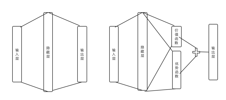
在Dueling DQN中，后面加了两个子网络结构，分别对应上面上到价格函数网络部分和优势函数网络部分。对应上面右图所示。最终Q网络的输出由价格函数网络的输出和优势函数网络的输出线性组合得到。

为了辨识两部分函数各自的作用，实际使用的组合公式如下：

$$Q(S,A,w,\alpha ,\beta )=V(S,w,\alpha )+\left(A(S,A,w,\beta )-\frac{1}{\mathcal{A}}\sum _{a^{\prime }\in \mathcal{A}}A(S,a^{\prime },w,\beta )\right)$$

Cartpole案例对偶DQN代码

这里我们重点关注Dueling DQN和Nature DQN的代码的不同之处。也就是网络结构定义部分，主要的代码如下，一共有两个相同结构的Q网络，每个Q网络都有状态函数和优势函数的定义，以及组合后的Q网络输出，主要是idden layer for state value和hidden layer for action value及Q Value layer的部分

def create_Q_network(self):
    # input layer
    self.state_input = tf.placeholder("float", [None, self.state_dim])
    # network weights
    with tf.variable_scope('current_net'):
        W1 = self.weight_variable([self.state_dim,20])
        b1 = self.bias_variable([20])

        # hidden layer 1
        h_layer_1 = tf.nn.relu(tf.matmul(self.state_input,W1) + b1)

        # hidden layer  for state value
        with tf.variable_scope('Value'):
          W21= self.weight_variable([20,1])
          b21 = self.bias_variable([1])
          self.V = tf.matmul(h_layer_1, W21) + b21

        # hidden layer  for action value
        with tf.variable_scope('Advantage'):
          W22 = self.weight_variable([20,self.action_dim])
          b22 = self.bias_variable([self.action_dim])
          self.A = tf.matmul(h_layer_1, W22) + b22

          # Q Value layer
          self.Q_value = self.V + (self.A - tf.reduce_mean(self.A, axis=1, keep_dims=True))

    with tf.variable_scope('target_net'):
        W1t = self.weight_variable([self.state_dim,20])
        b1t = self.bias_variable([20])

        # hidden layer 1
        h_layer_1t = tf.nn.relu(tf.matmul(self.state_input,W1t) + b1t)

        # hidden layer  for state value
        with tf.variable_scope('Value'):
          W2v = self.weight_variable([20,1])
          b2v = self.bias_variable([1])
          self.VT = tf.matmul(h_layer_1t, W2v) + b2v

        # hidden layer  for action value
        with tf.variable_scope('Advantage'):
          W2a = self.weight_variable([20,self.action_dim])
          b2a = self.bias_variable([self.action_dim])
          self.AT = tf.matmul(h_layer_1t, W2a) + b2a

          # Q Value layer
          self.target_Q_value = self.VT + (self.AT - tf.reduce_mean(self.AT, axis=1, keep_dims=True))

---

20241103

• 晚上仍然试跑30K，但还是力不能支，5K@349+1.2K@349+5K@354+2K@359，只能说差强人意。
  

• 现在感觉又是个瓶颈期，综合实力肯定不及上半年。一个是节奏不行，自从上半年伤后，350以外的配速我都不太适应用前脚掌跑，觉得垂直振幅大，很费劲，但是X3P这双鞋设计来就是用前掌跑，导致现在越跑越别扭。另一个是压不住速度，起手总是跑到350以内，然后自我感觉还很良好，心率蹭蹭得涨，三四公里之后就不太行了，坚持不了长距离。

• 第二个5K带的XR，本来前2K很稳定的410，感觉很轻松，结果这家伙很快就不行了，慢慢他就加到350以内冲掉了，后面我也是只能顶到5K。最后2K带的YY，起手420，本来还想补个10K的，但是他昨天被白辉龙榨干了，两圈人就没影了，后面我也感觉心肺扛不太住，也便是2K就冲掉了。

• 还剩两周，最后一周肯定是要减量，所以接下来一周是最后挣扎的时间了，感觉可能又是看临场发挥了。

• 战报：

  • 首先，2009级经济的李朝松又双叒叕PB了！两周前刚突破232达标一级，今天北马又以2:30:48成功PB一分钟，简直太夸张了。

  • 然后，2013级金融的孙大伟，北马净时间2:59:59极限破三，运气太好了，他成为了上财第十位破三的校友，而且看起来2004级财管的刘守征很可能会成为下一个破三的人选，而我还在苦苦挣扎，属实难绷。

  • 小崔市运会1500米摔了一跤还跑了4分39秒，只比嘉伟校运会慢3秒，顶级天赋，伟大，无需多言，但这次市运会前八门槛是4分29秒。他跟白辉龙注定成为接下来的双子星，上财中长跑未来的希望。

  • HJY女子800米2分49秒，不如去年的2分47秒，但也进前八了；DGL的1500米不知道跑了多少，这也是她最后一次了，她之后也不准备再练了，我觉得6分钟以内应该问题不大吧，但是对手很强，同济的两个都能跑到5分10秒以内，太夸张了。

  • 其余似乎没有很突出的成绩，不过今年北马确实很多人都PB了，可能有幸存者偏差的缘故，但估计确实是天时地利人和都在，陈龙、房博，都如愿跑进220达标健将了，大正也PB了，比柏林快十几秒大概。

关于位置编码的排列不变性与排列等变性

• input embedding + encoder + decoder
  • position encoding is in input embedding
• rnn 天然编码了位置信息
  • $h_t=f(h_{t-1},x_t)$
  • $f$ 是非线性激活函数，$h_{t-1}$ 是前一时间步的隐藏状态，$x_t$ 是当前时间步的输入。由于 $h_t$ 依赖于 $h_{t-1}$，而 $h_{t-1}$ 又依赖于 $h_{t-2}$，以此类推，隐藏状态包含了从初始时间步到当前时间步的所有历史信息。这种递归结构使得位置信息被隐式地编码在隐藏状态中。
  • RNN 通过其递归结构隐式地编码位置信息，而 Transformer 需要通过显式添加位置编码来获取位置信息。
• 如果在 Transformer Encoder 中没有使用位置编码，那么模型将无法区分输入序列中各个词的顺序，这实际上等同于一个词袋（Bag of Words）模型。原因是 Transformer 的自注意力机制本质上是对输入的加权求和，而没有位置编码的情况下，模型无法获取任何位置信息。
• Permutation Equivariance（排列等变）
  • Permutation Equivariance（排列等变）：如果对输入序列进行某种排列，模型的输出将以相同的方式被排列。
  • Permutation Invariance（排列不变）：对输入序列的排列不会影响模型的输出，即输出与输入的排列无关。
  • 没有位置编码的 Transformer Encoder 并不是排列不变的，而是排列等变的。这意味着如果我们改变输入序列中词的顺序，输出序列中的元素也会按照相同的方式重新排列，但输出本身的数值不会保持不变。

import torch
import torch.nn as nn
torch.manual_seed(42)
# 定义模型参数
vocab_size = 10000  # 词汇表大小
d_model = 512       # 嵌入维度
nhead = 8           # 注意力头数
num_layers = 1      # Transformer Encoder 层数

# RNN

# 定义输入序列
sequence_length = 5  # 序列长度
embedding_dim = 8    # 词嵌入维度
batch_size = 1       # 批大小
original_sequence = torch.randn(batch_size, sequence_length, embedding_dim)
original_sequence.shape # torch.Size([1, 5, 8])
original_sequence
"""
tensor([[[ 1.9269,  1.4873,  0.9007, -2.1055,  0.6784, -1.2345, -0.0431,
          -1.6047],
         [-0.7521,  1.6487, -0.3925, -1.4036, -0.7279, -0.5594, -0.7688,
           0.7624],
         [ 1.6423, -0.1596, -0.4974,  0.4396, -0.7581,  1.0783,  0.8008,
           1.6806],
         [ 0.0349,  0.3211,  1.5736, -0.8455,  1.3123,  0.6872, -1.0892,
          -0.3553],
         [-1.4181,  0.8963,  0.0499,  2.2667,  1.1790, -0.4345, -1.3864,
          -1.2862]]])
"""
permuted_sequence = original_sequence.clone()
permutation = torch.randperm(sequence_length)
permuted_sequence = permuted_sequence[:, permutation, :]
permuted_sequence.shape # torch.Size([1, 5, 8])
permuted_sequence
"""
tensor([[[ 1.9269,  1.4873,  0.9007, -2.1055,  0.6784, -1.2345, -0.0431,
          -1.6047],
         [-0.7521,  1.6487, -0.3925, -1.4036, -0.7279, -0.5594, -0.7688,
           0.7624],
         [-1.4181,  0.8963,  0.0499,  2.2667,  1.1790, -0.4345, -1.3864,
          -1.2862],
         [ 0.0349,  0.3211,  1.5736, -0.8455,  1.3123,  0.6872, -1.0892,
          -0.3553],
         [ 1.6423, -0.1596, -0.4974,  0.4396, -0.7581,  1.0783,  0.8008,
           1.6806]]])
"""
hidden_dim = 8
rnn = nn.RNN(input_size=embedding_dim, hidden_size=hidden_dim, batch_first=True)
ori_output, _ = rnn(original_sequence)
perm_output, _ = rnn(permuted_sequence)
ori_output.shape, perm_output.shape # (torch.Size([1, 5, 8]), torch.Size([1, 5, 8]))
# global mean pooling
ori_output.squeeze(0).mean(dim=0) # tensor([-0.2083,  0.0781, -0.1784,  0.0027,  0.2188,  0.4131,  0.1809, -0.0833], grad_fn=<MeanBackward1>)
perm_output.squeeze(0).mean(dim=0)
"""
tensor([-0.0615,  0.0666, -0.1055,  0.0008,  0.3712,  0.2399,  0.1625,  0.1277],
       grad_fn=<MeanBackward1>)
"""

---

20241104

• 又是被wyl气晕的下午，周日答辩，不知道最后这活能给他整成啥样。

• 嘉伟给我找了个好活，周四下午带五月姐和她师弟跑30K，五月姐要求30K@4’55"，她师弟则是30K@4’15"（看来这位也是奔着破三去练的，4’15"刚好是全马破三的配速），刚好他们两位也是在备赛南京马拉松，我也正愁没人一起跑30K，真是想睡觉就来枕头。

• DGL很贴心地给我同步了市运会成绩，4×400接力第四（4’58"，人均75秒以内），虽然3000米比校运会慢了10秒，但1500米5’40"可以说是非常超预期了，比去年要快17秒。两项都刚好是第八名，算是实力和运气都到位了。同济的黄芳1500米5’11"，3000米11’07"，人比人气死人。

• 有点被激励到，DGL上个月练得极其可怕，虽然我没去健身房，但是一周好像都要去练两三次负重深蹲，组数相当多，平时又是马不停蹄地间歇和以赛代练，能跑出这种成绩是情理之中了。

• PS：本来今天想补下肢力量训练，最后还是十点去实验楼负一层跳绳和跳台阶了（国教不知道在田径场搞什么飞机，搭了一堆棚子不让进），500次台阶交替步+1700次单摇+200次双摇+200次台阶交替步，结束左右各100次提踵拉伸，全是练的小腿和脚踝。国庆之后就一直没做下肢力量的训练，已经断了快一个月，想想可能现在慢跑前掌总感觉支撑不了，原因还是力量不足。

w/o pe

self_attention(perm(x)) = perm(self_attention(x)).

• x: input sequence
• perm：permutation，置换

# 定义嵌入层和 Transformer Encoder
embedding = nn.Embedding(vocab_size, d_model)
# dropout == 0.
encoder_layer = nn.TransformerEncoderLayer(d_model=d_model, nhead=nhead, dropout=0.0)
transformer_encoder = nn.TransformerEncoder(encoder_layer, num_layers=num_layers)

# 生成随机输入序列
seq_len = 10  # 序列长度
input_ids = torch.randint(0, vocab_size, (seq_len,))

# 打乱输入序列
perm = torch.randperm(seq_len)
shuffled_input_ids = input_ids[perm]

perm, torch.argsort(perm)
"""
(tensor([8, 3, 6, 4, 9, 5, 1, 2, 7, 0]),
 tensor([9, 6, 7, 1, 3, 5, 2, 8, 0, 4]))
"""

# 获取嵌入表示
embedded_input = embedding(input_ids)  # [seq_len, d_model]
embedded_shuffled_input = embedding(shuffled_input_ids)

# Transformer 期望的输入形状为 [seq_len, batch_size, d_model]，因此需要调整维度。

# 添加 batch 维度
# [seq_len, 1, d_model]
embedded_input = embedded_input.unsqueeze(1)           
embedded_shuffled_input = embedded_shuffled_input.unsqueeze(1)

# 通过 Transformer Encoder
output = transformer_encoder(embedded_input)           # [seq_len, 1, d_model]
output_shuffled = transformer_encoder(embedded_shuffled_input)

output.shape, output_shuffled.shape # (torch.Size([10, 1, 512]), torch.Size([10, 1, 512]))

torch.allclose(output, output_shuffled, atol=1e-6) # False
are_outputs_equal = torch.allclose(output.squeeze(1).mean(dim=0), output_shuffled.squeeze(1).mean(dim=0), atol=1e-6)
are_outputs_equal # True

inverse_perm = torch.argsort(perm)
output_shuffled_reordered = output_shuffled[inverse_perm]
torch.allclose(output, output_shuffled_reordered, atol=1e-6) # True

证明两者的结果相同，是不变的。

with pe

# 定义位置编码
class PositionalEncoding(nn.Module):
    def __init__(self, d_model, max_len=5000):
        super().__init__()
        # 创建位置编码矩阵
        position = torch.arange(0, max_len).unsqueeze(1)
        div_term = torch.exp(torch.arange(0, d_model, 2) * (-torch.log(torch.tensor(10000.0)) / d_model))
        pe = torch.zeros(max_len, 1, d_model)
        pe[:, 0, 0::2] = torch.sin(position * div_term)
        pe[:, 0, 1::2] = torch.cos(position * div_term)
        self.pe = pe

    def forward(self, x):
        # 加性位置编码
        x = x + self.pe[:x.size(0)]
        return x

# 添加位置编码
pos_encoder = PositionalEncoding(d_model)
embedded_input_pos = pos_encoder(embedded_input)
embedded_shuffled_input_pos = pos_encoder(embedded_shuffled_input)

# 通过 Transformer Encoder
output_pe = transformer_encoder(embedded_input_pos)
output_shuffled_pe = transformer_encoder(embedded_shuffled_input_pos)

output_pe.shape, output_shuffled_pe.shape # (torch.Size([10, 1, 512]), torch.Size([10, 1, 512]))

# global mean pooling
torch.allclose(output_pe.squeeze(1).mean(dim=0), output_shuffled_pe.squeeze(1).mean(dim=0), atol=1e-6) # False

下面我们重点证明：self_attention(perm(x)) = perm(self_attention(x))

P = torch.tensor([[1, 0, 0, 0],
                   [0, 0, 1, 0],
                   [0, 1, 0, 0],
                   [0, 0, 0, 1]])
P @ P.T, P.T @ P

• 设 $P$ 是排列矩阵，排列后的输入为：$X_{\text{perm}}=PX$
• QKV
  • $Q_{\text{perm}}=PQ,K_{\text{perm}}=PK,V_{\text{perm}}=PV$
• attention score matrix
  • $S_{\text{perm}}=\frac{Q_{\text{perm}}{K}_{\text{perm}}^T}{\sqrt{d_k}}=\frac{PQ{K}^T{P}^T}{\sqrt{d_k}}=P\left(\frac{Q{K}^T}{\sqrt{d_k}}\right)P^T=PS{P}^T$
    • $S=\frac{Q{K}^T}{\sqrt{d_k}}$
• softmax
  • $A_{\text{perm}}=\text{softmax}(S_{\text{perm}})=\text{softmax}(PS{P}^T)=PA{P}^T$
    • $A=\text{softmax(S)}$
• attention output
  • $Y_{\text{perm}}=A_{\text{perm}}{V}_{\text{perm}}=PA{P}^{T}PV=P(AV)$
    • 对于排列矩阵 $P^{T}P=I$

import torch.nn.functional as F

P = torch.tensor([[1, 0, 0, 0],
                   [0, 0, 1, 0],
                   [0, 1, 0, 0],
                   [0, 0, 0, 1]], dtype=torch.float32)
S = torch.randn(4, 4)

F.softmax(P @ S @ P.T, dim=1), P @ F.softmax(S, dim=1) @ P.T
"""
(tensor([[0.0658, 0.0774, 0.1272, 0.7297],
         [0.1882, 0.7317, 0.0716, 0.0085],
         [0.7313, 0.0426, 0.1071, 0.1191],
         [0.1295, 0.3200, 0.1981, 0.3524]]),
 tensor([[0.0658, 0.0774, 0.1272, 0.7297],
         [0.1882, 0.7317, 0.0716, 0.0085],
         [0.7313, 0.0426, 0.1071, 0.1191],
         [0.1295, 0.3200, 0.1981, 0.3524]]))
"""

---

20241105

• 晚饭后，小腿开始有点胀，最近确实是练少了，之前力量训练之后都不会有什么感觉。

• 今晚一共10K（2K@405+5K@422+3K@401），起手跑了2K看到嘉伟跟韬哥在慢摇，真的特别慢，居然5分多的配速在摇，而且摇了有十几公里，我说嘉伟你耐心真好，遂停下来陪他俩也摇了两公里。

• 后来看到一个特专业的装备哥，穿的莫干山越野的衣服，跑姿和身材都很好，追上前去问他是不是学生，然后哥们儿一回头，才发现是马桢。

• 其实我还是没认出来（脸盲），因为之前并不认识他，校运会那天他来参加5000米才认识，但他一直在群里，是AX拉进来的，之前就听说是个越野大佬，不可小觑，5000米赛前问他能跑多少，他说估计按3’45"的配速来跑吧，暗暗称奇，结果他跑崩了，19’44"排名第八。跑完跟AX合照比了个❤，我说你俩好gay啊，两个大男人还搁这比心，他说年轻人真的猛（第三白辉龙都把他都套了一圈多，AX应该是险些套到他圈，反正我是没被嘉伟套到圈的），我估计他可能比AX还要大一些，比白辉龙大了得有10岁，想想跑不赢比自己小10岁的小朋友，到底还是不太服气的。

• PS：依然跑得很笨重，尽管心率不高。可能还是到晚上太疲劳了，很想能再放慢一些堆一堆量，但是时间已经很紧了，又不敢比马配更慢，若是连马配都觉得吃力，那还怎么破三？有些无奈。
  

w/o pe

self_attention(perm(x)) = perm(self_attention(x)).

• x: input sequence
• perm：permutation，置换

# 定义嵌入层和 Transformer Encoder
embedding = nn.Embedding(vocab_size, d_model)
# dropout == 0.
encoder_layer = nn.TransformerEncoderLayer(d_model=d_model, nhead=nhead, dropout=0.0)
transformer_encoder = nn.TransformerEncoder(encoder_layer, num_layers=num_layers)

# 生成随机输入序列
seq_len = 10  # 序列长度
input_ids = torch.randint(0, vocab_size, (seq_len,))

# 打乱输入序列
perm = torch.randperm(seq_len)
shuffled_input_ids = input_ids[perm]

perm, torch.argsort(perm)
"""
(tensor([8, 3, 6, 4, 9, 5, 1, 2, 7, 0]),
 tensor([9, 6, 7, 1, 3, 5, 2, 8, 0, 4]))
"""

# 获取嵌入表示
embedded_input = embedding(input_ids)  # [seq_len, d_model]
embedded_shuffled_input = embedding(shuffled_input_ids)

# Transformer 期望的输入形状为 [seq_len, batch_size, d_model]，因此需要调整维度。

# 添加 batch 维度
# [seq_len, 1, d_model]
embedded_input = embedded_input.unsqueeze(1)           
embedded_shuffled_input = embedded_shuffled_input.unsqueeze(1)

# 通过 Transformer Encoder
output = transformer_encoder(embedded_input)           # [seq_len, 1, d_model]
output_shuffled = transformer_encoder(embedded_shuffled_input)

output.shape, output_shuffled.shape # (torch.Size([10, 1, 512]), torch.Size([10, 1, 512]))

torch.allclose(output, output_shuffled, atol=1e-6) # False
are_outputs_equal = torch.allclose(output.squeeze(1).mean(dim=0), output_shuffled.squeeze(1).mean(dim=0), atol=1e-6)
are_outputs_equal # True

inverse_perm = torch.argsort(perm)
output_shuffled_reordered = output_shuffled[inverse_perm]
torch.allclose(output, output_shuffled_reordered, atol=1e-6) # True

证明两者的结果相同，是不变的。

with pe

# 定义位置编码
class PositionalEncoding(nn.Module):
    def __init__(self, d_model, max_len=5000):
        super().__init__()
        # 创建位置编码矩阵
        position = torch.arange(0, max_len).unsqueeze(1)
        div_term = torch.exp(torch.arange(0, d_model, 2) * (-torch.log(torch.tensor(10000.0)) / d_model))
        pe = torch.zeros(max_len, 1, d_model)
        pe[:, 0, 0::2] = torch.sin(position * div_term)
        pe[:, 0, 1::2] = torch.cos(position * div_term)
        self.pe = pe

    def forward(self, x):
        # 加性位置编码
        x = x + self.pe[:x.size(0)]
        return x

# 添加位置编码
pos_encoder = PositionalEncoding(d_model)
embedded_input_pos = pos_encoder(embedded_input)
embedded_shuffled_input_pos = pos_encoder(embedded_shuffled_input)

# 通过 Transformer Encoder
output_pe = transformer_encoder(embedded_input_pos)
output_shuffled_pe = transformer_encoder(embedded_shuffled_input_pos)

output_pe.shape, output_shuffled_pe.shape # (torch.Size([10, 1, 512]), torch.Size([10, 1, 512]))

# global mean pooling
torch.allclose(output_pe.squeeze(1).mean(dim=0), output_shuffled_pe.squeeze(1).mean(dim=0), atol=1e-6) # False

下面我们重点证明：self_attention(perm(x)) = perm(self_attention(x))

P = torch.tensor([[1, 0, 0, 0],
                   [0, 0, 1, 0],
                   [0, 1, 0, 0],
                   [0, 0, 0, 1]])
P @ P.T, P.T @ P

• 设 $P$ 是排列矩阵，排列后的输入为：$X_{\text{perm}}=PX$
• QKV
  • $Q_{\text{perm}}=PQ,K_{\text{perm}}=PK,V_{\text{perm}}=PV$
• attention score matrix
  • $S_{\text{perm}}=\frac{Q_{\text{perm}}{K}_{\text{perm}}^T}{\sqrt{d_k}}=\frac{PQ{K}^T{P}^T}{\sqrt{d_k}}=P\left(\frac{Q{K}^T}{\sqrt{d_k}}\right)P^T=PS{P}^T$
    • $S=\frac{Q{K}^T}{\sqrt{d_k}}$
• softmax
  • $A_{\text{perm}}=\text{softmax}(S_{\text{perm}})=\text{softmax}(PS{P}^T)=PA{P}^T$
    • $A=\text{softmax(S)}$
• attention output
  • $Y_{\text{perm}}=A_{\text{perm}}{V}_{\text{perm}}=PA{P}^{T}PV=P(AV)$
    • 对于排列矩阵 $P^{T}P=I$

import torch.nn.functional as F

P = torch.tensor([[1, 0, 0, 0],
                   [0, 0, 1, 0],
                   [0, 1, 0, 0],
                   [0, 0, 0, 1]], dtype=torch.float32)
S = torch.randn(4, 4)

F.softmax(P @ S @ P.T, dim=1), P @ F.softmax(S, dim=1) @ P.T
"""
(tensor([[0.0658, 0.0774, 0.1272, 0.7297],
         [0.1882, 0.7317, 0.0716, 0.0085],
         [0.7313, 0.0426, 0.1071, 0.1191],
         [0.1295, 0.3200, 0.1981, 0.3524]]),
 tensor([[0.0658, 0.0774, 0.1272, 0.7297],
         [0.1882, 0.7317, 0.0716, 0.0085],
         [0.7313, 0.0426, 0.1071, 0.1191],
         [0.1295, 0.3200, 0.1981, 0.3524]]))
"""

---

20241106

• 大美兴，川普王！这是大学之后经历的第三次大选，每次都是不同的结局。第一次，谁都不看好他，然后他莫名其妙赢了，双方还算体面；第二次，谁都看好他，然后他输了，他表现得很不体面；第三次，不管谁赢，结局都不会体面了。前期谁都看好他，然后他中弹，对手换帅，局势又很莫名其妙地变得焦灼，明明双方根本就不是一个量级的对手，哈哈姐在懂王面前不就是个小卡拉米么？虽然台上可能只是棋子，输赢的关键并不在他们，但是这种完全不对等的对决实在有些滑稽。

• 又是被wyl折磨一整天，今天估计又要弄到十二点。晚上九点摇了5K渐加速@417，前半程心率很低，一直不到150bpm，后面突然变得有些艰难，不太能搞得清一点。尽管最近午睡都跟猪一样死，但是到晚上还是疲劳得很，不过明天带五月姐他们跑完，五月姐请吃长白山烤肉，一下有动力了。
  

transformers细节全记录（一）

import torch
from torch import nn
import torch.nn.functional as F
import numpy as np
import pandas as pd
import matplotlib.pyplot as plt
import matplotlib as mpl
from IPython.display import Image
# default: 100
mpl.rcParams['figure.dpi'] = 150

torch.manual_seed(42)

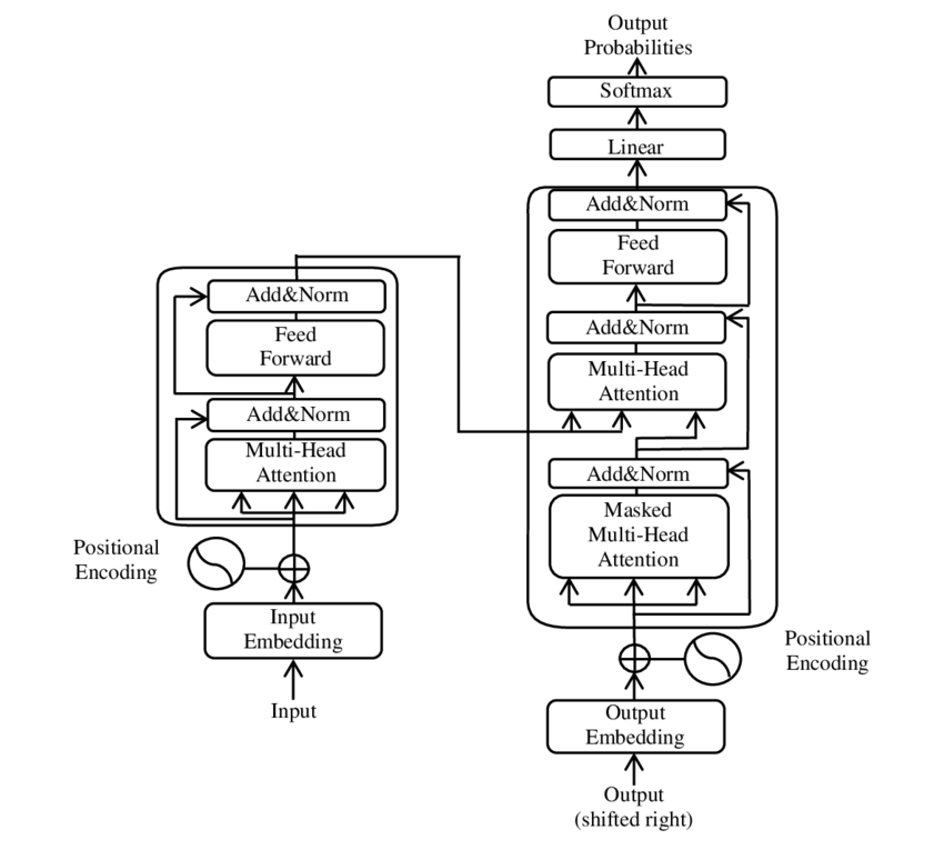
• pytorch transformer (seq modeling) => transformers (hf, focus on language models) => LLM
• pytorch
  • nn.TransformerEncoderLayer => nn.TransformerEncoder
    • TransformerEncoder is a stack of N encoder layers.
    • BERT
  • nn.TransformerDecoderLayer => nn.TransformerDecoder
    • TransformerDecoder is a stack of N decoder layers.
    • GPT
• decoder 与 encoder 相比，有两个特殊的 attention sublayers
  • masked multi-head (self) attention
  • encoder-decoder (cross) attention
    • (k, v) from encoder （memory, last encoder layer）
    • q：decoder input
    • multihead_attn(x, mem, mem) from TransformerDecoderLayer
  • 两者权值不共享

(masked) multi-head attention

https://pytorch.org/docs/stable/generated/torch.nn.functional.scaled_dot_product_attention.html

• Encoder Self-Attention:
  • No Masking:
    • Since attn_bias is zero, the attention weights depend solely on the scaled dot product:
      $${\text{Scores}}_{\text{encoder}}=\frac{Q{K}^{\top }}{\sqrt{d_k}}$$
      $${\text{Attention}}_{\text{encoder}}=\text{softmax}({\text{Scores}}_{\text{encoder}})$$
    • Each token attends to all tokens, including future ones.
• Decoder Masked Self-Attention:
  • Causal Masking:
    • The mask M is defined as:
      $$M_{i,j}=\{\begin{array}{ll}0& \text{if }j\le i\\ -\infty & \text{if }j>i\end{array}$$
    • The attention scores become:
      $${\text{Scores}}_{\text{decoder}}=\frac{Q{K}^{\top }}{\sqrt{d_k}}+M$$
    • Applying softmax:
      $${\text{Attention}}_{\text{decoder}}=\text{softmax}({\text{Scores}}_{\text{decoder}})$$
      • The -inf in M ensures that positions where ( j > i ) (future positions) have zero attention weight.

---

20241107

• 最近确实点背，之前手机进水，今天为了算一道随机过程的题，翻草稿纸抬手就把水杯的水洒在键盘上，把大一就跟着我的拯救者笔记本给整没了，只听风扇呼啸一声，屏幕直接变雪花，估计是主板烧坏了。虽然八九年也不是很心疼，里面也没存啥有用的东西，坏就坏了吧。

• 下午带五月姐跟她师弟张鹏跑长距离，课表是21K@4’10"，嘉伟带五月姐30K@5’10"，两个人都圆满的完成了课表，实力确实强，五月姐万米PB是40分台，他们这些群体都是有私人教练，严格按照课表系统训练，的确不是我们这些半吊子跑者能比的。

• 但是我还是没想到张鹏竟然这么强，83年的老哥，上市公司高管，一年前还是个200斤的胖子，结果现在居然有这种水平。他们都叫他卷王，月跑量400K以上，今天也是从闵行开车来训练，太勤奋了。

  • 起手4K张鹏鞋带开了，我稍微等了他几秒钟，很快我意识到他的呼吸很喘，以为他顶不住这个配速，但他说前15K都可以按这个节奏来，于是我也就没有放水。之后都是严格按照4’10"以内的配速带他，他到12K之后每一圈都要去拿水喝，偶尔补胶（我全程是没有任何补给的，因为不习惯补给，节奏容易乱），感觉他随时都有可能要崩，结果他愣是一直坚挺到21K，最后2K甚至提速到4分以内，把我都给拉爆了，让我特别吃惊。

• 今天状态还是可以的，前18K节奏很稳，并没有吃力感，而且心率超级低，大部分时候都在160bpm以下，从心率水平上来说甚至超越了三月巅峰期的表现。但是小腿还是有点胀，用的还是前掌跑，到后程我感觉脚踝有点不适，想改成后跟跑法，但是一用后跟跑小腿就要抽筋（前掌跑是压迫小腿，后跟跑是拉伸小腿），根本不能改跑姿，就硬生生前掌跑完了20K（我少跑1K，因为真的是被他拉爆了），后来感觉右脚内侧稍微有一点点抽筋，但是不至于像上半年那次伤痛那么厉害。

• 总之接下来以休整为主，赛前大概率不会再拉20K以上的距离了，虽然我真的还缺一个30K，但是现在还是尽量低强度过渡，把疲劳的身体恢复过来。

• PS：怎么说呢，需要一些运气，平心而论，今天训练的表现真的不算差了，但20K这个阈值不知道该如何跨过，很难想象跑完一个半马之后还要再跑一个半马，不掉速几乎不可能。遗憾没能在状态最巅峰的时期跑完首马，现在破三的把握不足两成。
  

transformers细节全记录（二）

encoder layer & encoder

• input: $\mathbf{X}\in {\mathbb{R}}^{T\times B\times d_{\text{model}}}$
• 1. multihead selfattn
  • 线性变换（linear projection, 矩阵乘法）生成 Q、K、V矩阵
  • $X_{\text{flat}}=\mathbf{X}.\text{reshape}(T\times B,d_{model})$
  • $\mathbf{QKV}=\mathbf{X}{\mathbf{W}}_{in}^T+{\mathbf{b}}_{in}$（encoder_layer.self_attn.in_proj_weight, encoder_layer.self_attn.in_proj_bias）
    • ${\mathbf{W}}_{in}\in {\mathbb{R}}^{3d_{\text{model}}\times d_{\text{model}}}$，${\mathbf{b}}_{in}\in {\mathbb{R}}^{3d_{\text{model}}}$
    • $\mathbf{QKV}\in {\mathbb{R}}^{T\times B,3d_{model}}$
  • 拆分 $\mathbf{Q},\mathbf{K},\mathbf{V}$
    • $\mathbf{Q},\mathbf{K},\mathbf{V}=\text{split}(\mathbf{QKV},d_{model})$（按列进行拆分）
    • $\mathbf{Q},\mathbf{K},\mathbf{V}\in {\mathbb{R}}^{T\times B,d_{\text{model}}}$
  • 调整形状以适应多头注意力
    • $d_k=\frac{d_{\text{model}}}{h}$
    • reshape_for_heads
      $$\begin{array}{rl}{\mathbf{Q}}_{\text{heads}}& =\mathbf{Q}.\text{reshape}(T,B,h,d_k).\text{permute}(1,2,0,3).\text{reshape}(B\times h,T,d_k)\\ {\mathbf{K}}_{\text{heads}}& =\mathbf{K}.\text{reshape}(T,B,h,d_k).\text{permute}(1,2,0,3).\text{reshape}(B\times h,T,d_k)\\ {\mathbf{V}}_{\text{heads}}& =\mathbf{V}.\text{reshape}(T,B,h,d_k).\text{permute}(1,2,0,3).\text{reshape}(B\times h,T,d_k)\end{array}$$
  • 计算注意力分数：$\text{Scores}=\frac{{\mathbf{Q}}_{\text{heads}}{\mathbf{K}}_{\text{heads}}^{\top }}{\sqrt{d_k}}$
    • ${\mathbf{Q}}_{\text{heads}}\in {\mathbb{R}}^{(B\times h)\times T\times d_k}$，${\mathbf{K}}_{\text{heads}}^{\top }\in {\mathbb{R}}^{(B\times h)\times d_k\times T}$，因此 $\text{Scores}\in {\mathbb{R}}^{(B\times h)\times T\times T}$。
  • 计算注意力权重：$\text{AttentionWeights}=\text{softmax}(\text{Scores})$
  • 计算注意力输出：$\text{AttentionOutput}=\text{AttentionWeights}\times {\mathbf{V}}_{\text{heads}}$
    • ${\mathbf{V}}_{\text{heads}}\in {\mathbb{R}}^{(B\times h)\times T\times d_k}$，因此 $\text{AttentionOutput}\in {\mathbb{R}}^{(B\times h)\times T\times d_k}$。
  • 合并多头输出：$\text{AttentionOutput}=\text{AttentionOutput}.\text{reshape}(B,h,T,d_k).\text{permute}(2,0,1,3).\text{reshape}(T,B,d_{\text{model}})$
  • 输出线性变换：$\text{AttnOutputProjected}=\text{AttentionOutput}{\mathbf{W}}_{\text{out}}^{\top }+{\mathbf{b}}_{\text{out}}$
    • ${\mathbf{W}}_{\text{out}}\in {\mathbb{R}}^{d{}_{\text{model}}\times d_{\text{model}}}$，${\mathbf{b}}_{\text{out}}\in {\mathbb{R}}^{d_{\text{model}}}$，对应代码中的out_proj_weight和out_proj_bias。
• 2. 残差连接和层归一化（第一层）
  • 残差连接：$\text{Residual1}=\mathbf{X}+\text{AttnOutputProjected}$
  • 层归一化：$\text{Normalized1}=\text{LayerNorm}(\text{Residual1},{\gamma }_{\text{norm1}},{\beta }_{\text{norm1}})$
    • ${\gamma }_{\text{norm1}},{\beta }_{\text{norm1}}\in {\mathbb{R}}^{d_{\text{model}}}$，对应代码中的norm1.weight 和 norm1.bias。
• 3. 前馈神经网络 (ffn)
  • 第一层线性变换和激活函数：$\text{FFNOutput1}=\text{ReLU}(\text{Normalized1}{\mathbf{W}}_1^{\top }+{\mathbf{b}}_1)$
    • 其中，${\mathbf{W}}_1\in {\mathbb{R}}^{d_{\text{ff}}\times d_{\text{model}}}$，${\mathbf{b}}_1\in {\mathbb{R}}^{d_{\text{ff}}}$，对应代码中的 linear1.weight 和linear1.bias。
  • 第二层线性变换：$\text{FFNOutput2}=\text{FFNOutput1}{\mathbf{W}}_2^{\top }+{\mathbf{b}}_2$
    • 其中，${\mathbf{W}}_2\in {\mathbb{R}}^{d_{\text{model}}\times d_{\text{ff}}}$，${\mathbf{b}}_2\in {\mathbb{R}}^{d_{\text{model}}}$，对应代码中的 linear2.weight 和 linear2.bias。
• 4. 残差连接和层归一化（第二层）
  • 残差连接：$\text{Residual2}=\text{Normalized1}+\text{FFNOutput2}$
  • 层归一化：$\text{Output}=\text{LayerNorm}(\text{Residual2},{\gamma }_{\text{norm2}},{\beta }_{\text{norm2}})$
    • 其中，${\gamma }_{\text{norm2}},{\beta }_{\text{norm2}}\in {\mathbb{R}}^{d_{\text{model}}}$，对应代码中的 norm2.weight 和 norm2.bias。

d_model = 4  # 模型维度
nhead = 2    # 多头注意力中的头数
dim_feedforward = 8  # 前馈网络的维度
batch_size = 1
seq_len = 3

assert d_model % nhead == 0
encoder_input = torch.randn(seq_len, batch_size, d_model)  # [seq_len, batch_size, d_model]
# 禁用 droput
encoder_layer = nn.TransformerEncoderLayer(d_model=d_model, nhead=nhead,
                                           dim_feedforward=dim_feedforward, dropout=0.0)
                                           memory = encoder_layer(encoder_input)  # 编码器输出
memory
"""
tensor([[[-1.0328, -0.9185,  0.6710,  1.2804]],
        [[-1.4175, -0.1948,  1.3775,  0.2347]],
        [[-1.0022, -0.8035,  0.3029,  1.5028]]],
       grad_fn=<NativeLayerNormBackward0>)
"""
encoder_input.shape, memory.shape # (torch.Size([3, 1, 4]), torch.Size([3, 1, 4]))

---

20241108

• 昨晚11点多临走前，发现操场灯火通明，凑近一看，一群人在跑道上骑车，我直接震惊，上个月某个周六早上我也见过他们，师傅还特意正装出席给他们清场，这帮人后台挺硬。

• 忍不了一点，开喷。且不论田径场能不能骑车，我近距离看过他们的身材和装备，不说TT了，都是些死飞甚至还有山地车，不是哥们，就这配置也要来田径场训练？去健身房把大腿练粗些，租不起自行车竞速场地，附近清流环一二路一整天都很空旷，大半夜在学校浪费资源来装X是真受不了一点。

• 右脚足弓内侧的确是扭到了，是去年扬马扭伤的位置，走路有点瘸，大概不会疼太久。考虑到今晚保守估计要开会到十点半，晚饭后去操场想练会儿。偶遇嘉伟慢跑，他说明年上半年会再冲击一回全马245，这个冬训估计会好好堆有氧。我实在跑不起来，补了30箭步×8组（+20kg），试着拉了几个引体，身体好重。

• PS：感觉AX和LXY有戏诶，我也觉得挺合适。

Transformer细节全记录（三）

手写encoder

encoder_layer = nn.TransformerEncoderLayer(d_model=d_model, nhead=nhead,
                                           dim_feedforward=dim_feedforward, dropout=0.0)

形如：

TransformerEncoderLayer(
  (self_attn): MultiheadAttention(
    (out_proj): NonDynamicallyQuantizableLinear(in_features=4, out_features=4, bias=True)
  )
  (linear1): Linear(in_features=4, out_features=8, bias=True)
  (dropout): Dropout(p=0.0, inplace=False)
  (linear2): Linear(in_features=8, out_features=4, bias=True)
  (norm1): LayerNorm((4,), eps=1e-05, elementwise_affine=True)
  (norm2): LayerNorm((4,), eps=1e-05, elementwise_affine=True)
  (dropout1): Dropout(p=0.0, inplace=False)
  (dropout2): Dropout(p=0.0, inplace=False)
)

调整模型输入的形状

X = encoder_input  # [3, 1, 4]
X_flat = X.contiguous().view(-1, d_model)  # [T * B, d_model] -> [3, 4]

多层注意力层

self_attn = encoder_layer.self_attn
# d_model = 4
# (3d_model, d_model), (3d_model)
self_attn.in_proj_weight.shape, self_attn.in_proj_bias.shape # (torch.Size([12, 4]), torch.Size([12]))
# d_model = 4
# (d_model, d_model), (d_model) 
self_attn.out_proj.weight.shape, self_attn.out_proj.bias.shape # (torch.Size([4, 4]), torch.Size([4]))

W_in = self_attn.in_proj_weight
b_in = self_attn.in_proj_bias

W_out = self_attn.out_proj.weight
b_out = self_attn.out_proj.bias

QKV = F.linear(X_flat, W_in, b_in)  # [3, 3*d_model]
QKV.shape # torch.Size([3, 12])

Q, K, V = QKV.split(d_model, dim=1)  # 每个维度为[3, d_model]
Q.shape, K.shape, V.shape # (torch.Size([3, 4]), torch.Size([3, 4]), torch.Size([3, 4]))

# 调整Q、K、V的形状以适应多头注意力
head_dim = d_model // nhead  # 每个头的维度
def reshape_for_heads(x):
    return x.contiguous().view(seq_len, batch_size, nhead, head_dim).permute(1, 2, 0, 3).reshape(batch_size * nhead, seq_len, head_dim)

Q = reshape_for_heads(Q)
K = reshape_for_heads(K)
V = reshape_for_heads(V)
# B*h, T, d_k
Q.shape, K.shape, V.shape # (torch.Size([2, 3, 2]), torch.Size([2, 3, 2]), torch.Size([2, 3, 2]))

# 计算注意力分数
scores = torch.bmm(Q, K.transpose(1, 2)) / (head_dim ** 0.5)  # [batch_size * nhead, seq_len, seq_len]

# 应用softmax
attn_weights = F.softmax(scores, dim=-1)  # [batch_size * nhead, seq_len, seq_len]

# 计算注意力输出
attn_output = torch.bmm(attn_weights, V)  # [batch_size * nhead, seq_len, head_dim]

# 调整形状以合并所有头的输出
attn_output = attn_output.view(batch_size, nhead, seq_len, head_dim).permute(2, 0, 1, 3).contiguous()
attn_output = attn_output.view(seq_len, batch_size, d_model)  # [seq_len, batch_size, d_model]

# 通过输出投影层
attn_output = F.linear(attn_output.view(-1, d_model), W_out, b_out)  # [seq_len * batch_size, d_model]
attn_output = attn_output.view(seq_len, batch_size, d_model)

这里我们看一下atten_weights.sum(dim=-1)

tensor([[1.0000, 1.0000, 1.0000],
        [1.0000, 1.0000, 1.0000]], grad_fn=<SumBackward1>)

即就是一个加权平均

残差连接和层归一化（第一层）

norm1 = encoder_layer.norm1
residual = X + attn_output  # [seq_len, batch_size, d_model]
normalized = F.layer_norm(residual, (d_model,), weight=norm1.weight, bias=norm1.bias)  # [seq_len, batch_size, d_model]

通过前馈神经网络：

W_1 = encoder_layer.linear1.weight
b_1 = encoder_layer.linear1.bias

W_2 = encoder_layer.linear2.weight
b_2 = encoder_layer.linear2.bias

norm2 = encoder_layer.norm2

ffn_output = F.linear(normalized.view(-1, d_model), W_1, b_1)  # [seq_len * batch_size, dim_feedforward]
ffn_output = F.relu(ffn_output)  # [seq_len * batch_size, dim_feedforward]

# 第二层线性变换
ffn_output = F.linear(ffn_output, W_2, b_2)  # [seq_len * batch_size, d_model]
ffn_output = ffn_output.view(seq_len, batch_size, d_model)  # [seq_len, batch_size, d_model]

# 残差连接和层归一化（第二层）
residual2 = normalized + ffn_output  # [seq_len, batch_size, d_model]
normalized2 = F.layer_norm(residual2, (d_model,), weight=norm2.weight, bias=norm2.bias)  # [seq_len, batch_size, d_model]
normalized2
"""
tensor([[[-1.0328, -0.9185,  0.6710,  1.2804]],

        [[-1.4175, -0.1948,  1.3775,  0.2347]],

        [[-1.0022, -0.8035,  0.3029,  1.5028]]],
       grad_fn=<NativeLayerNormBackward0>)
"""
torch.allclose(normalized2, memory) # True

---

20241109

• 昨晚还是保守了，wyl直接六个多小时开到今天。

• 回血日，右脚的扭伤还是有点重，走几百米就特别疼，情况类似去年扬马之前，疼得位置也一样，去年清明节，我跟宋某训练，意外扭到右脚，当时觉得不碍事，两三天就好了，然后两周后的扬马旧伤复发走了7K，脚肿得跟鸡蛋一样。有预感这次会是历史重演，但是不可能这时候再放弃了。

• 我都想最后一周直接不训练，就跑休到赛前，一天最多两三公里，说不定效果会更好。我并不担心伤痛，一来，已经轻车熟路，多次伤痛，更严重的都挺过来了；二来，反正跑完就回扬州躺着了，对我来说南马这一战是破釜沉舟，之后日子不过了。

• PS：下午白辉龙20个400米@80秒，间歇1分钟，小崔330-400的变速10K，年轻就是好啊。AK今早世纪公园35K@3’56"，极其强势的表现，他真有可能今年要跑进240，而且他昨天翘了我订的酒店（本来是他之前说要跟我一起住的），所以我有理由怀疑他南马是不是要带家属来，之前他说南马就4分配顺下来，上马再发力，看这样子估计是南马就要发力了；SXY雁荡山山脊线20K，一口气1000米的爬升，直上直下，有点厉害的。

transformer细节全记录（四）

解码器部分

• input: $\mathbf{Y}\in {\mathbb{R}}^{T\times B\times d_{\text{model}}}$（解码器输入）

• memory: $\mathbf{M}\in {\mathbb{R}}^{T_{\text{enc}}\times B\times d_{\text{model}}}$（编码器输出）

• 1. Multi-head Self-Attention（解码器的多头自注意力）
  • 线性变换（linear projection，矩阵乘法）生成 ${\mathbf{Q}}_{\text{self}}$、${\mathbf{K}}_{\text{self}}$、${\mathbf{V}}_{\text{self}}$ 矩阵
    • $Y_{\text{flat}}=\mathbf{Y}.\text{reshape}(T\times B,d_{\text{model}})$
    • ${\mathbf{QKV}}_{\text{self}}=Y_{\text{flat}}{\mathbf{W}}_{\text{in,self}}^{\top }+{\mathbf{b}}_{\text{in,self}}$（decoder_layer.self_attn.in_proj_weight，decoder_layer.self_attn.in_proj_bias）
      • ${\mathbf{W}}_{\text{in,self}}\in {\mathbb{R}}^{3d_{\text{model}}\times d_{\text{model}}}$，${\mathbf{b}}_{\text{in,self}}\in {\mathbb{R}}^{3d_{\text{model}}}$
      • ${\mathbf{QKV}}_{\text{self}}\in {\mathbb{R}}^{T\times B,3d_{\text{model}}}$
    • 拆分 ${\mathbf{Q}}_{\text{self}}$、${\mathbf{K}}_{\text{self}}$、${\mathbf{V}}_{\text{self}}$
      • ${\mathbf{Q}}_{\text{self}}$, ${\mathbf{K}}_{\text{self}}$, ${\mathbf{V}}_{\text{self}}=\text{split}({\mathbf{QKV}}_{\text{self}},d_{\text{model}})$（按列进行拆分）
      • ${\mathbf{Q}}_{\text{self}}$, ${\mathbf{K}}_{\text{self}}$, ${\mathbf{V}}_{\text{self}}\in {\mathbb{R}}^{T\times B,d_{\text{model}}}$
  • 调整形状以适应多头注意力
    • $d_k=\frac{d_{\text{model}}}{h}$
    • reshape_for_heads
      $$\begin{array}{rl}{\mathbf{Q}}_{\text{heads,self}}& ={\mathbf{Q}}_{\text{self}}.\text{reshape}(T,B,h,d_k).\text{permute}(1,2,0,3).\text{reshape}(B\times h,T,d_k)\\ {\mathbf{K}}_{\text{heads,self}}& ={\mathbf{K}}_{\text{self}}.\text{reshape}(T,B,h,d_k).\text{permute}(1,2,0,3).\text{reshape}(B\times h,T,d_k)\\ {\mathbf{V}}_{\text{heads,self}}& ={\mathbf{V}}_{\text{self}}.\text{reshape}(T,B,h,d_k).\text{permute}(1,2,0,3).\text{reshape}(B\times h,T,d_k)\end{array}$$
  • 计算注意力分数：${\text{Scores}}_{\text{self}}=\frac{{\mathbf{Q}}_{\text{heads,self}}{\mathbf{K}}_{\text{heads,self}}^{\top }}{\sqrt{d_k}}$
    • ${\mathbf{Q}}_{\text{heads,self}}\in {\mathbb{R}}^{(B\times h)\times T\times d_k}$，${\mathbf{K}}_{\text{heads,self}}^{\top }\in {\mathbb{R}}^{(B\times h)\times d_k\times T}$，因此 ${\text{Scores}}_{\text{self}}\in {\mathbb{R}}^{(B\times h)\times T\times T}$
  • （可选）应用遮掩矩阵
    • 如果需要应用遮掩（例如防止解码器看到未来的信息），生成遮掩矩阵 $\text{Mask}\in {\mathbb{R}}^{T\times T}$
    • 对 ${\text{Scores}}_{\text{self}}$ 应用遮掩：${\text{Scores}}_{\text{self}}={\text{Scores}}_{\text{self}}+\text{Mask}$
  • 计算注意力权重：${\text{AttentionWeights}}_{\text{self}}=\text{softmax}({\text{Scores}}_{\text{self}})$
  • 计算注意力输出：${\text{AttentionOutput}}_{\text{self}}={\text{AttentionWeights}}_{\text{self}}\times {\mathbf{V}}_{\text{heads,self}}$
    • ${\mathbf{V}}_{\text{heads,self}}\in {\mathbb{R}}^{(B\times h)\times T\times d_k}$，因此 ${\text{AttentionOutput}}_{\text{self}}\in {\mathbb{R}}^{(B\times h)\times T\times d_k}$
  • 合并多头输出：${\text{AttentionOutput}}_{\text{self}}={\text{AttentionOutput}}_{\text{self}}.\text{reshape}(B,h,T,d_k).\text{permute}(2,0,1,3).\text{reshape}(T,B,d_{\text{model}})$
  • 输出线性变换：${\text{AttnOutputProjected}}_{\text{self}}={\text{AttentionOutput}}_{\text{self}}{\mathbf{W}}_{\text{out,self}}^{\top }+{\mathbf{b}}_{\text{out,self}}$
    • ${\mathbf{W}}_{\text{out,self}}\in {\mathbb{R}}^{d_{\text{model}}\times d_{\text{model}}}$，${\mathbf{b}}_{\text{out,self}}\in {\mathbb{R}}^{d_{\text{model}}}$，对应代码中的 self_out_proj_weight 和 self_out_proj_bias
• 2. 残差连接和层归一化（第一层）
  • 残差连接：$\text{Residual1}=\mathbf{Y}+{\text{AttnOutputProjected}}_{\text{self}}$
  • 层归一化：$\text{Normalized1}=\text{LayerNorm}(\text{Residual1},{\gamma }_{\text{norm1}},{\beta }_{\text{norm1}})$
    • ${\gamma }_{\text{norm1}},{\beta }_{\text{norm1}}\in {\mathbb{R}}^{d_{\text{model}}}$，对应代码中的 norm1.weight 和 norm1.bias
• 3. Multi-head Encoder-Decoder Attention（交叉注意力）
  • 线性变换生成 ${\mathbf{Q}}_{\text{cross}}$、${\mathbf{K}}_{\text{cross}}$、${\mathbf{V}}_{\text{cross}}$ 矩阵
    • 对于查询矩阵：
      • ${\mathbf{Q}}_{\text{cross}}={\text{Normalized1}}_{\text{flat}}{\mathbf{W}}_{\text{q,cross}}^{\top }+{\mathbf{b}}_{\text{q,cross}}$
        • ${\mathbf{W}}_{\text{q,cross}}\in {\mathbb{R}}^{d_{\text{model}}\times d_{\text{model}}}$，${\mathbf{b}}_{\text{q,cross}}\in {\mathbb{R}}^{d_{\text{model}}}$
    • 对于键和值矩阵：
      • ${\mathbf{KV}}_{\text{cross}}=M_{\text{flat}}{\mathbf{W}}_{\text{k,v,cross}}^{\top }+{\mathbf{b}}_{\text{k,v,cross}}$
        • ${\mathbf{W}}_{\text{k,v,cross}}\in {\mathbb{R}}^{2d_{\text{model}}\times d_{\text{model}}}$，${\mathbf{b}}_{\text{k,v,cross}}\in {\mathbb{R}}^{2d_{\text{model}}}$
      • 拆分 ${\mathbf{K}}_{\text{cross}}$, ${\mathbf{V}}_{\text{cross}}$
        • ${\mathbf{K}}_{\text{cross}}$, ${\mathbf{V}}_{\text{cross}}=\text{split}({\mathbf{KV}}_{\text{cross}},d_{\text{model}})$
  • 调整形状以适应多头注意力
    • reshape_for_heads
      $$\begin{array}{rl}{\mathbf{Q}}_{\text{heads,cross}}& ={\mathbf{Q}}_{\text{cross}}.\text{reshape}(T,B,h,d_k).\text{permute}(1,2,0,3).\text{reshape}(B\times h,T,d_k)\\ {\mathbf{K}}_{\text{heads,cross}}& ={\mathbf{K}}_{\text{cross}}.\text{reshape}(T_{\text{enc}},B,h,d_k).\text{permute}(1,2,0,3).\text{reshape}(B\times h,T_{\text{enc}},d_k)\\ {\mathbf{V}}_{\text{heads,cross}}& ={\mathbf{V}}_{\text{cross}}.\text{reshape}(T_{\text{enc}},B,h,d_k).\text{permute}(1,2,0,3).\text{reshape}(B\times h,T_{\text{enc}},d_k)\end{array}$$
    • 注意：$T_{\text{enc}}$ 是编码器输出的序列长度
  • 计算注意力分数：${\text{Scores}}_{\text{cross}}=\frac{{\mathbf{Q}}_{\text{heads,cross}}{\mathbf{K}}_{\text{heads,cross}}^{\top }}{\sqrt{d_k}}$
    • ${\text{Scores}}_{\text{cross}}\in {\mathbb{R}}^{(B\times h)\times T\times T_{\text{enc}}}$
  • 计算注意力权重：${\text{AttentionWeights}}_{\text{cross}}=\text{softmax}({\text{Scores}}_{\text{cross}})$
  • 计算注意力输出：${\text{AttentionOutput}}_{\text{cross}}={\text{AttentionWeights}}_{\text{cross}}\times {\mathbf{V}}_{\text{heads,cross}}$
    • ${\text{AttentionOutput}}_{\text{cross}}\in {\mathbb{R}}^{(B\times h)\times T\times d_k}$
  • 合并多头输出：${\text{AttentionOutput}}_{\text{cross}}={\text{AttentionOutput}}_{\text{cross}}.\text{reshape}(B,h,T,d_k).\text{permute}(2,0,1,3).\text{reshape}(T,B,d_{\text{model}})$
  • 输出线性变换：${\text{AttnOutputProjected}}_{\text{cross}}={\text{AttentionOutput}}_{\text{cross}}{\mathbf{W}}_{\text{out,cross}}^{\top }+{\mathbf{b}}_{\text{out,cross}}$
    • ${\mathbf{W}}_{\text{out,cross}}\in {\mathbb{R}}^{d_{\text{model}}\times d_{\text{model}}}$，${\mathbf{b}}_{\text{out,cross}}\in {\mathbb{R}}^{d_{\text{model}}}$，对应代码中的 cross_out_proj_weight 和 cross_out_proj_bias
• 4. 残差连接和层归一化（第二层）
  • 残差连接：$\text{Residual2}=\text{Normalized1}+{\text{AttnOutputProjected}}_{\text{cross}}$
  • 层归一化：$\text{Normalized2}=\text{LayerNorm}(\text{Residual2},{\gamma }_{\text{norm2}},{\beta }_{\text{norm2}})$
    • ${\gamma }_{\text{norm2}},{\beta }_{\text{norm2}}\in {\mathbb{R}}^{d_{\text{model}}}$，对应代码中的 norm2.weight 和 norm2.bias
• 5. 前馈神经网络（FFN）
  • 第一层线性变换和激活函数：$\text{FFNOutput1}=\text{ReLU}(\text{Normalized2}{\mathbf{W}}_1^{\top }+{\mathbf{b}}_1)$
    • ${\mathbf{W}}_1\in {\mathbb{R}}^{d_{\text{ff}}\times d_{\text{model}}}$，${\mathbf{b}}_1\in {\mathbb{R}}^{d_{\text{ff}}}$，对应代码中的 linear1.weight 和 linear1.bias
  • 第二层线性变换：$\text{FFNOutput2}=\text{FFNOutput1}{\mathbf{W}}_2^{\top }+{\mathbf{b}}_2$
    • ${\mathbf{W}}_2\in {\mathbb{R}}^{d_{\text{model}}\times d_{\text{ff}}}$，${\mathbf{b}}_2\in {\mathbb{R}}^{d_{\text{model}}}$，对应代码中的 linear2.weight 和 linear2.bias
• 6. 残差连接和层归一化（第三层）
  • 残差连接：$\text{Residual3}=\text{Normalized2}+\text{FFNOutput2}$
  • 层归一化：$\text{Output}=\text{LayerNorm}(\text{Residual3},{\gamma }_{\text{norm3}},{\beta }_{\text{norm3}})$
    • ${\gamma }_{\text{norm3}},{\beta }_{\text{norm3}}\in {\mathbb{R}}^{d_{\text{model}}}$，对应代码中的 norm3.weight 和 norm3.bias

解码器实现类似编码器

---

20241110

• 犯太岁了是最近，印象中搬到三门路来五年没丢过各种钥匙跟卡。倒霉事真全凑一起了，先是手机和电脑进水报销，然后赛前十天把右脚弄伤，昨天又把车钥匙给弄丢了，昨晚回来找不到车钥匙连车都骑不了，被迫一瘸一拐走回三门路，真扎心了。

• 今天上午走路依然疼得厉害，但是到晚上已经不算太碍事，稍微注意一些走起来不会疼，但疼痛肯定是还没好。无碍。

• PS：后来我估摸着最近没车还是不行，毕竟还是半个残废，然后带着打气筒和扳手出去想找找看有没有废弃的车能用先，成功在新园门口找到一辆前后轮都瘪得没气的山地车（没锁），稍微修整了下，打个气就能骑了，虽然灰尘落了些，但是骑起来一点声音都没有，感觉是辆好车，有点罪恶感哈哈。反正先凑合一阵子呗，等我想办法把原来那辆车的锁给撬了先。

pytorch 高维张量 Tensor 维度操作与处理，einops

import torch
from torch import nn
import torch.nn.functional as F
import numpy as np
import pandas as pd

d = 4  # 模型维度
B = 2
T = 3
h = 2    # 多头注意力中的头数
ff = 8  # 前馈网络的维度

X = torch.randn(T, B, d)  # [seq_len, batch_size, d_model]
X.shape # torch.Size([3, 2, 4])
encoder = nn.TransformerEncoderLayer(d, h, ff, dropout=0.0)
W_in, b_in = encoder.self_attn.in_proj_weight, encoder.self_attn.in_proj_bias
# (3d, d), (3d, )
W_in.shape, b_in.shape # (torch.Size([12, 4]), torch.Size([12]))
encoder(X).shape # torch.Size([3, 2, 4])

1 张量内存

[pytorch] Tensor shape 变化 view 与 reshape（contiguous 的理解）)

https://stackoverflow.com/questions/26998223/what-is-the-difference-between-contiguous-and-non-contiguous-arrays

• 张量内存 layout
  • 在大多数深度学习框架（如 PyTorch）中，（高维）张量的数据是以一维数组的形式在内存中连续存储的。对于多维张量，其高维结构是通过一维内存数组和步幅（strides）来实现的。
  • pytorch 存储顺序（Storage Order）是 Row-major，最后一个维度变化最快。
• Strides（步幅）
  • 对于一个形状为 $(D_0,D_1,D_2)$（2*3*4） 的 3D 张量，其步幅计算如下：
    • $\text{stride[2]}=1$
    • $\text{stride[1]}=D_2\times \text{stride[2]}=D_2$ （3）
    • $\text{stride[0]}=D_1\times \text{stride[1]}=D_1\times D_2$（3*4=12）

A = torch.randint(0, 5, (2, 3, 4))
"""
tensor([[[0, 0, 3, 0],
         [3, 3, 1, 1],
         [0, 3, 1, 4]],

        [[1, 1, 0, 2],
         [4, 1, 1, 0],
         [4, 1, 0, 3]]])
"""

• 当张量在内存中的数据排列不再符合其形状和步幅之间的默认关系时，张量就是非连续的（is not contiguous）。
  • 特征：.is_contiguous() 方法返回 False。
  • 影响：某些操作在非连续张量上可能性能较差，或者需要额外的内存拷贝。
  • 解决方法：使用 .contiguous() 方法，将张量拷贝为内存中连续的版本。
• 什么样的操作会导致内存的不连续
  • permute, transpose, view;
    • transpose 是 permute 的特例，transpose 只允许交换两个维度。
• reshape 不改变内存中的数据顺序

A = torch.randn(3, 4)
A.shape, A.stride(), A.is_contiguous() # (torch.Size([3, 4]), (4, 1), True)
A = A.transpose(0, 1)
A.shape, A.stride(), A.is_contiguous() # (torch.Size([4, 3]), (1, 4), False)
A = A.contiguous()
A.shape, A.stride(), A.is_contiguous() # (torch.Size([4, 3]), (3, 1), True)

2 view v.s. reshape

• view（类比sql中的概念）
  • 不会复制数据：view 创建的是原始张量的一个新的视图，内存数据保持不变，只是重新解释内存中的数据。因为它依赖于张量的内存布局，所以无法对非连续的张量使用。
  • 不连续内存，view 时有可能报错；
• reshape: 它会自动处理非连续张量，尽可能返回视图，如果无法返回视图，则会拷贝
  • 不要求内存连续：reshape 可以用于非连续的张量。如果张量不连续，reshape 会自动尝试创建一个新的连续张量并复制数据，以确保能够完成形状转换。
  • 可能复制数据：当张量是内存不连续的，reshape 可能会进行数据复制，生成一个新的内存布局的张量。否则，它和 view 的行为是一样的，不复制数据。
  • 不改变数据在内存中的顺序，只改变张量的形状解释。

A = torch.randn(2, 3, 4)
A.view(-1, 4).shape, A.view(-1, 4).stride(), A.view(-1, 4).is_contiguous(), 
# (torch.Size([6, 4]), (4, 1), True)

A = torch.randn(2, 3, 4)
A_t = A.permute(1, 2, 0)
A.stride(), A_t.shape, A_t.stride(), A_t.is_contiguous()
# ((12, 4, 1), torch.Size([3, 4, 2]), (4, 1, 12), False)

---

20241111

• 找了把剪锁钳，居然剪不断锁，艹。

• 今天小崔也表演了30个400米间歇，77-81秒，间歇90秒。这俩人现在不知道算不算良性竞争，好疯狂。

• 停跑三天，晚上简单跑了2K，勉强能跑，但伤没有完全好，也不敢跑太多，但是一点不跑显然也不太行，到时候万一伤痛复发就退赛吧。最近韬哥倒是经常看到。

• 总要接受和承认技不如人。想想上半年已经很幸运了，能在状态最好的时期跑出了万米和半马的PB，可能以后再也跑不到那时候的水平，但人生能有多少逢其时呢，得失之间罢了。

• PS：没心没肺的人也会变诶，L，emmm

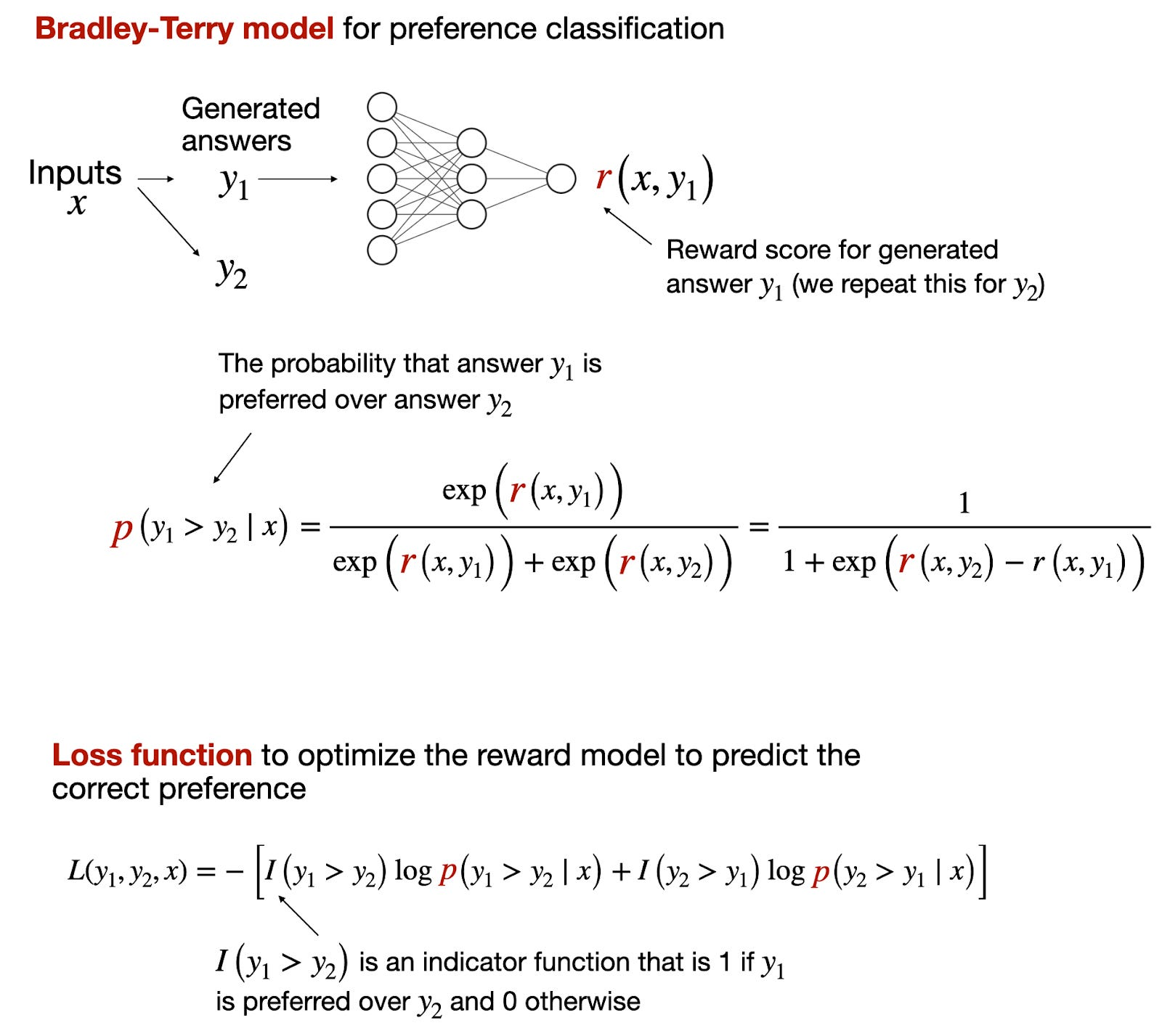
instructGPT 中的 reward modeling，概率建模与损失函数性质

• references
  • https://en.wikipedia.org/wiki/Bradley%E2%80%93Terry_model
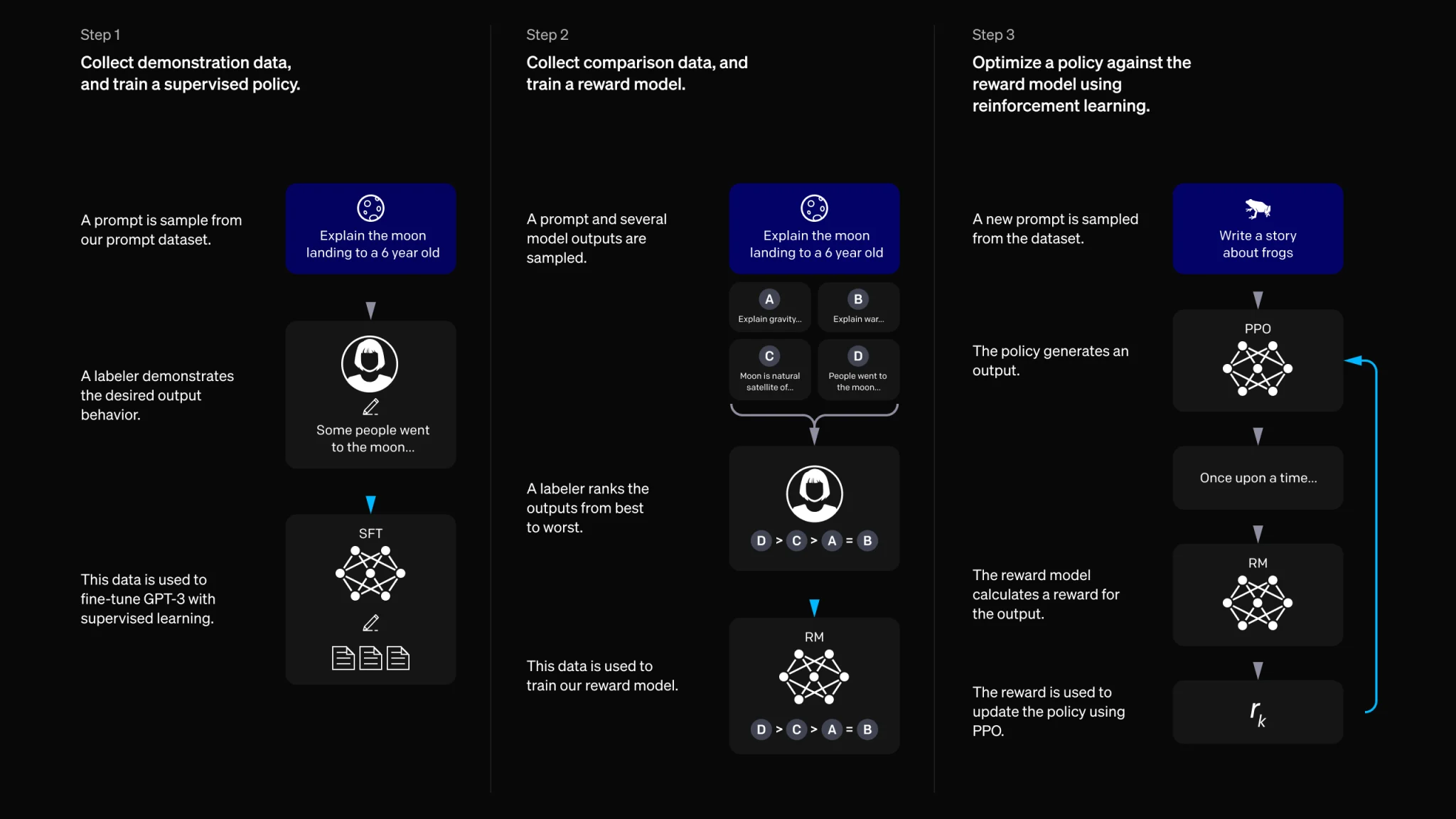
  • InstructGPT:
    • https://openai.com/index/instruction-following/
    • https://arxiv.org/abs/2203.02155（关于chatgpt完整介绍的文章）
    • 论文介绍了chatgpt训练的三阶段，第一阶段basemodel，第二阶段是reward model（人标不同输出的一个概率比值）

标注者的打分未必一致，但是偏序更可能是一致的

import torch
from torch import nn
import torch.nn.functional as F
import numpy as np
import matplotlib.pyplot as plt

1 instructGPT

$$\text{loss}(\theta )=-\frac{1}{\left(\genfrac{}{}{0ex}{}{K}{2}\right)}{\mathbb{E}}_{(x,y_w,y_l)\sim D}\left[\log \left(\sigma \left(r_{\theta }(x,y_w)-r_{\theta }(x,y_l)\right)\right)\right]$$

• D>C>A=B

• 单个的标注（监督学习，直接回归 rating），rating 未必是全局唯一的，
  • labeler A 认为的 3分在 labeler B 的 4分或者2分，即 rating 的 scale 未必对所有的 labelers 都是适用的；
  • 李克特量表（Likert scale）
• reward model
  • 双输入，siamese network；

1.1 损失函数的理解

1.2 概率建模

$$\begin{array}{rl}\delta =r_w-r_l& =\log odds=\log \frac{p}{1-p}\\ & \Downarrow \\ p& =\frac{1}{1+\exp (-\delta )}=\sigma (\delta )\\ & \Downarrow \\ & -\log p=-\log \sigma (\delta )\end{array}$$

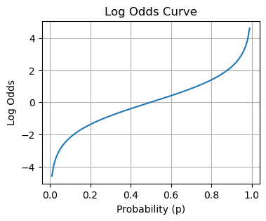
• log odds（对数赔率，赔率的对数）：$r_w-r_l=\log odds$
  • $p=p(y_w>y_l)$
  • 奖励差，表示人类更可能偏好响应1（$r_w$，$r_{\text{chosen}}$）而非响应2（$r_{\ell }$，$r_{\text{rejected}}$）的对数赔率。
• They use a cross-entropy loss, with the comparisons as labels—the difference in rewards represents the log odds that one response will be preferred to the other by a human labeler
  • 我们已经假定人类标注者更偏好响应1，设定真实标签 $y=1$；（如果人类更偏好响应2，设定 $y=0$）
  • 则交叉熵损失为 $-[y\log P+(1-y)\log (1-P)]=-\log P$
• 多数时候我们看到 log probability 的时候基本就是在计算交叉熵；

p = np.linspace(0.01, 0.99, 100)
log_odds = np.log(p / (1 - p))  # Calculate log odds

# Plotting the log odds curve
plt.figure(figsize=(4, 3))
plt.plot(p, log_odds)
plt.xlabel('Probability (p)')
plt.ylabel('Log Odds')
plt.title('Log Odds Curve')
plt.grid(True)

2 multiple responses

$$k=9$$

• 可以很大的膨胀数据集的规模
  • batch size 64，k = 9
  • $\le 64\cdot \left(\genfrac{}{}{0ex}{}{9}{2}\right)=2304$
• 这里取K=9，是考虑到人工标注的时候，很大一部分时间是花在读懂这个prompt。而读懂prompt和一两个答案之后，其它答案就理解的很快了。所以排序9个比排序4个所花的时间并不是增加了一倍。而且 $C_9^2=36,C_4^2=6$，等于额外开销不到一倍，而标注的数据多了6倍。
• 另外之前的工作不仅是 K=4 ，而且在标注的时候只标注最好的一个 ，这样就是4选1，这样只需要最大化最优答案的分数就行，所以容易过拟合。而这里采用的是
  $C_k^2$ 个排序对，使得整个问题变得复杂一点，缓解了过拟合，也能增加偏序数据对的数量

import math
64 * math.comb(9, 2) # 2304

3 Bradley-Terry model

梯度的损失：

$$\begin{array}{rl}& \ell =-\log \sigma (\delta )\\ & {\ell }^{\prime }=\sigma (\delta )-1\end{array}$$

• loss is proportional to the log odds that the first resp is greater than the second;

# `r1=r2` 时的 loss
-F.logsigmoid(torch.tensor(0.)), -np.log10(1/(1+np.exp(-0)))

import numpy as np
import matplotlib.pyplot as plt

# Define the delta range
delta = np.linspace(-10, 10, 1000)

# Define the function -log(sigma(delta)) and its gradient
sigma = 1 / (1 + np.exp(-delta))
neg_log_sigma = -np.log(sigma)
grad_neg_log_sigma = sigma-1  # derivative of -log(sigma(delta)) with respect to delta

# Plotting
plt.figure(figsize=(5, 3))
plt.plot(delta, neg_log_sigma, label='$-\log(\sigma(\delta))$', color='blue')
plt.plot(delta, grad_neg_log_sigma, label="Gradient of $-\log(\sigma(\delta))$", color='red', linestyle='--')

plt.axhline(0, color='black', linewidth=0.5, linestyle=':')
plt.axvline(0, color='black', linewidth=0.5, linestyle=':')

plt.title('Plot of $-log(\sigma(\delta))$ and its Gradient')
plt.xlabel('delta')
plt.ylabel('Function Value / Gradient')
plt.legend()
plt.grid(True)
plt.show()
# (tensor(0.6931), 0.3010299956639812)

• $\delta =r_1-r_2\ge 3$ 以后 loss 接近于0，且基本没有梯度了；

-np.log(1/(1+np.exp(-1))), -np.log(1/(1+np.exp(-3))), -np.log(1/(1+np.exp(-(-6))))
# -np.log(1/(1+np.exp(-1))), -np.log(1/(1+np.exp(-3))), -np.log(1/(1+np.exp(-(-6))))
1
-np.log(1/(1+np.exp(-1))), -np.log(1/(1+np.exp(-3))), -np.log(1/(1+np.exp(-(-6))))
(0.3132616875182228, 0.0485873515737419, 6.00247568513773)

1/(1+np.exp(-(-6))) # 0.0024726231566347743

---

20241112

• 足弓内侧那个点的疼痛还是消不掉，一朝被蛇咬，十年怕井绳，因为跟去年疼的位置一模一样，真是有心理阴影。今晚马配跑了5K也没啥事，穿的还是风衣长裤+代步鞋，但也不是说就真就没事了，因为去年也是同样的情况，赛前十天受伤，到赛前三天（周四）感觉好了，那天晚上跟嘉伟410左右跑到7K，脚又出问题。

  • 去年的时间线：4月5日下午初次扭伤，到4月13日晚二次扭伤，4月16日扬马，从热身就已经感觉疼，起跑1公里上文昌大桥就已经疼得很厉害，到14K停下走路，平山堂路连续的上下坡折磨得脚完全受不了，后面又硬拖着走了7K，但是即便如此，4月25日我还是把校运会5000米跑下来了（20’50"第五）。

• 状态肯定是不如之前，心率很高，两三公里就感觉有些喘了。毕竟快一周没怎么好好跑，但欲速不达，急着跑，到时候再伤也得不偿失，上半年临阵脱逃，这次再放弃实在说不过去了。

• PS：八点半去操场路上刚好三教下晚课，路上全是人，人群中杀出一个LXY，飞快。
  

[AI硬件科普] 内存/显存带宽，从 NVIDIA 到苹果 M4

https://www.bilibili.com/video/BV1Y9DAYwEvg

内存带宽（memory bandwidth），内存位宽（memory bus width）

一些显卡的数据可以在wikipedia找：https://en.wikipedia.org/wikiAmpere/(microarchitecture}

• 内存带宽计算公式：

  • 内存带宽 = 频率 * 位宽/8

• 内存频率：MT/s(GT/s) 与 Gbps

  • MT/s：Mega Transfers per Second
    • MT/s 表示每秒的传输次数。
      • 如果每次传输传输 1 位的数据，那么 1 MT/s = 1 Mbps。
      • 如果每次传输传输的是 8 位（即 1 字节）的数据，那么 1 MT/s = 8 Mbps。
  • Gbps：Gigabits per Second

• NVIDIA GeForce RTX 4090：

  • 显存类型：24 GB GDDR6X。
  • 显存位宽：384 位。
  • 显存频率：21 Gbps。

• A100：显存位宽达到了 5120位；

  • 显存类型：HBM（high bandwidth memory）

• M4 series

  • https://en.wikipedia.org/wiki/Apple_M4
  • M4：LPDDR5X 7500 MT/s
    • 内存位宽：64bit*2 = 128位 (16*8)
      • 2表示的RAM的双通道；
    • 内存带宽计算：
      • 7500*64*2/8/1000 = 120GB/s
  • M4 pro/max：LPDDR5X 8533 MT/s
    • M4 pro：
      • 内存位宽：64bit * 4 = 256bits (16 * 16)
        • 4 表示的 RAM 的4通道
      • 内存带宽
        • 8533 * 64 * 4 / 8 / 1000 = 273GB/s
    • M4 max：
      • 内存位宽：128 * {3, 4} = {384, 512}bits (24 * 16, 32 * 16)
        • 3 表示的 RAM 的 3 通道（3颗粒）；
      • 内存带宽：
        • 8533 * 128 * 3 / 8 / 1000 = 410 GB/s
        • 8533 * 128 * 4 / 8 / 1000 = 546 GB/s

f'{21 * 384 / 8}GB/s' # '1008.0GB/s'
7500 * 64*2 / 8 / 1000 # 120.0
8533 * 64 * 4 / 8 / 1000 # 273.056
8533 * 128 * 3 / 8 / 1000 # 409.584
128 * 4 # 512
8533 * 128 * 4 / 8 / 1000 # 546.112

• 内存带宽似乎也能追上相对高端的GPU芯片；
• 核心数量和整体并行计算能力上与专门的深度学习 GPU（如 NVIDIA A100 或 H100）相比存在差距。
  • cuda、cuda cores
• 专用硬件加速：NVIDIA 和其他高端 GPU 提供 Tensor Cores 等专用单元，加速矩阵运算和深度学习的计算效率。这些特性在 M4 Max 上可能无法完全匹配。

内存通道

• 内存的非对称双通道，笔记本电脑一般两个内存通道（双通道内存）
  • 比如一根16gb内存跟一根8gb内存，
  • 如果想16gb升级成24gb
    • 原厂一根16gb，然后再买一个 8gb
    • 如果原厂是两根8gb，则需要买一根16gb替换其中一根8gb

segment fault (core dump)

“Segment fault (core dumped)” 是程序运行时的一个错误，通常发生在程序试图访问未被允许的内存区域时。它是由操作系统通过内存保护机制检测到的，并终止程序执行，同时产生一个内存转储文件（即 core dump），用于调试。

---

[工具使用] tmux 会话管理及会话持久性

• 终端复用器（terminal multiplexer）
• 安装：sudo apt-get install tmux
  • tmux -V
• 进入 tmux 模式：terminal 中输入 tmux 回车
  • Ctrl +b：激活控制台
    • "：上下
    • %：左右
    • o：切换窗口；
    • x：关闭当前窗口；

!tmux -V

显示 # tmx 3.2a

Session会话管理：

• 创建会话：tmux new -s 0827
  • 比如启动某服务
• 退出会话：ctrl + b -> d（detatch）
• 进入会话：tmux attach -t 0827
  • -t：target
• 查看会话：
  • tmux ls

其他操作：

• 设置鼠标触摸板支持
  • tmux set mouse on
• tmux attach -t 3

---

[A100 02] GPU 服务器压力测试，gpu burn，cpu burn，cuda samples

• 两种方式

  • 源码：https://github.com/wilicc/gpu-burn

  git clone https://github.com/wilicc/gpu-burn
  cd gpu-burn
  make
  ./gpu_burn
  ./gpu_burn 60
  ./gpu_burn -tc 300 (major >= 7)
  

  • tar.gz：http://wili.cc/blog/gpu-burn.html

  tar -zxvf xx.tar.gz -C
  cd xx
  make
  

• 也可以指定卡去跑

export CUDA_VISIBLE_DEVICES=1
./gpu_burn 100

• 4090 (tc)
  • 2.7% proc'd: 880 (145963 Gflop/s) - 880 (146466 Gflop/s) errors: 0 - 0 temps: 46 C - 46 C
• 3090ti (tc)
  • 55350 Gflop/s
• A100-40GB (tc)
  • 100.0% proc'd: 32568 (118649 Gflop/s) - 33534 (122261 Gflop/s) errors: 0 - 0

cpuburn

• https://patrickmn.com/projects/cpuburn/

  • 解压直接 ./cpuburn;

  Burning 152 CPUs/cores
  

  • 测试cpu传感器温度

  # 安装
  sudo apt install lm-sensors
  # 配置，yes
  sudo sensors-detect
  watch -n 1 sensors
  # 也可以查看系统监视器（system monitor）
  

cuda-samples

# 安装 cmake
sudo apt install cmake -y

git clone https://github.com/NVIDIA/cuda-samples.git
# git clone git@github.com:NVIDIA/cuda-samples.git
cd cuda-samples
# git checkout tags/v12.0
# conda deactivate
make

• references

  • https://docs.nvidia.com/cuda/demo-suite/index.html

• cuda-samples/Samples/1_Utilities/

  • deviceQuery：设备查询；
  • bandwidthTest：测试带宽；
    • ./bandwidthTest -device=all

• cuda-samples/Samples/5_Domain_Specific/

  • p2pBandwidthLatencyTest：两块gpu，卡间p2p带宽；
  • P2P技术允许两个GPU直接相互通信，而不需要通过CPU

deviceQuery

• cuda driver version / runtime version
• cuda capability major/minor version number
• cuda cores
  • 4090: 16384 cuda cores, A100: 6912
• memory bus width
  • 4090: 384-bit, A100: 5120-bit

from fractions import Fraction
Fraction(16384, 6912) # Fraction(64, 27)
16384 / 6912 # 2.370370370370370

bandwithTest（带宽测试）

• 不同类型的内存传输
  • 主机到设备（host to device，即CPU及其内存传输到设备（GPU内存））
  • 设备到主机（device to host，从设备（GPU内存）回传到主机（系统内存））
  • 设备到设备（device to device，两个GPU之间直接传输数据的性能）

1080ti

---

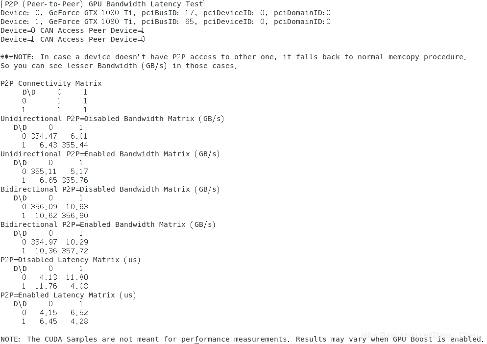
[A100 01] A100 服务器开箱，超微平台，gpu、cpu、内存、硬盘等信息查看

• 参考资料
  • https://infohub.delltechnologies.com/static/media/client/7phukh/DAM_d6ac0280-3398-47e3-8ad8-075751746a0b.pdf
  • https://nigelcannings.medium.com/unlocking-maximum-inference-capability-a-deep-dive-into-llama2-70b-on-an-80gb-a100-gpu-2ab1158d6b0b

配置清单

• 超微（supermicro）7049GP原厂平台
  • https://www.youtube.com/watch?v=C-ygJ3bcMSs
  • Dual-socket Intel Xeon Scalable
  • Support up to 4X GPUs
  • 2U/4U 表示的是平放时的高度；
• 处理器（CPU）的至强铂金 8374B *2 总计 76核心 152线程
  • 至强铂金：Xeon Platinum
• 内存是 ddr4 3200MHZ 64G*8根 =512G
• 显卡是 Nvidia A100-40GB * 2
  • PCI-e, nvlink
• 硬盘是 三星 2T M.2 NVME

gpus

• Nvidia A100-40GB，

• nvidia-smi topo -p2p p

• nvidia-smi topo -m

• https://www.youtube.com/watch?v=flxBD-YwXmM

  • NVIDIA NVLink Bridge 3-Slot on NVIDIA RTX A6000
    • NVLink桥接器的物理尺寸和所需的插槽空间

cpu

• lscpu

  • Socket(s): CPU插槽（物理CPU）的数量，表述 CPU 的物理插槽；
  • CPU(s): 显示逻辑CPU的总数。(152) （nproc: the number of processing units available）
  • On-line CPU(s) list: 在线的CPU编号列表。(0-151)

• 注意区别核心数（Cores，物理的）和线程数（Threads，逻辑的，逻辑处理线程，是操作系统能够进行调度的最小执行单元。）

  • CPU(s): 显示逻辑CPU的总数，总的线程数；
    • 152
  • Core(s) per socket: 这个数字表示每个CPU插槽（socket）中的核心数（Cores）
    • 38
  • Thread(s) per core: 这个数字表示每个核心支持的线程数。
  • 38*2*2 = 152

其他

• 内存条（RAM）：内存可选得话 ddr4 3200MHZ 规格的： 16G 32G 64G 128G 256G都可以

  • 可以插16根

• sudo dmidecode --type memory

• sudo dmidecode --type memory | grep -i type

• sudo dmidecode --type memory | grep -i size

• sudo dmidecode --type memory | grep -i speed

• free -h：使用情况

• 硬盘：nvme 的安装（https://www.youtube.com/shorts/2s34x-mt1wk）

  • lsblk：
    • /dev/nvme0n1p1:
      • nvme 表示设备使用NVMe协议，
      • 0 通常是指控制器编号，
      • n1 表示第一个NVMe设备（n后面的数字代表设备编号），
      • 而p1 表示设备的第一个分区（p后面的数字代表分区编号）。
        • /dev/nvme0n1p2
    • 查看操作系统安装所在的磁盘分区
      • findmnt -n -o SOURCE /
  • df -h：磁盘使用情况
  • 查看硬盘品牌及型号

  sudo apt install smartmontools
  sudo smartctl -a /dev/nvme0n1p1 | grep Model
  

---

20241113

• 剪了个寸头，背水一战。

• 晚饭后去操场消食，本来没打算跑多少，衣服鞋子也没换，但是跑着跑着就4分半出头跑了10K，如果不是这双鞋太磨脚，可以摇到天荒地老。

• 自上周四20K跑完，停跑三天，接着最近三天循序渐进稍微上了些量，总之肯定是能跑的，但是破三的希望不大。就这么慢慢摇真的很舒服，但其实也不能跑得太多，今天跑完之后，足弓那个点还是很疼的，跑着的时候疼得不明显，一旦停下来就相当难受。如果是按破三去跑，估计八成甚至九成是要退赛，而且很可能是重伤退场；但如果只是按4分半出头的配速去跑，有七成把握能顺利完赛，这样也是至少3小时20分以内的成绩了，其实不算差。

  • 可是，3小时20分对我来说跟3小时01分似乎也没有区别，我就是很执拗地想首马破三。

• 唉，可能到时候还是会去拼一拼的，大概吧。现在真的随便抬腿就能跑到410以内，怎么甘心就这么认怂呢？还有不到四天，还是有一点点希望能完全康复的？

• PS：老妈说肯定是要来南京的，其实她主要目的并不是来看我，其实我也不太想她来南京。不过老妈昨天刚逼老爸去隔壁做胃肠镜，把息肉给开掉，老爸在家休息一周也没啥事，如果我真的再次受伤，也能开车把我带回去，省得一瘸一拐再一路折磨走一路了。
  

[显卡驱动] lspci 显卡是否在槽位，显卡基本信息

• nvcc

  • 有可能的路径是 ~/anaconda3/bin/nvcc

• 注意 nvidia driver 与 cuda 是两个不同的东西

  • 先安装 dirver 再安装 cuda，两者的版本关系是：https://docs.nvidia.com/cuda/cuda-toolkit-release-notes/index.html

1 驱动问题

NVIDIA-SMI has failed because it couldn’t communicate with the NVIDIA driver. Make sure that the latest NVIDIA driver is installed and running.

显卡是否在槽位（显卡有没有掉）

!lspci | grep -i nvidia

18:00.0 VGA compatible controller: NVIDIA Corporation Device 2684 (rev a1)
18:00.1 Audio device: NVIDIA Corporation Device 22ba (rev a1)
8a:00.0 VGA compatible controller: NVIDIA Corporation Device 2684 (rev a1)
8a:00.1 Audio device: NVIDIA Corporation Device 22ba (rev a1)

• 一共2个GPU，每个GPU都有一个相应的VGA兼容控制器和一个音频设备。
  • NVIDIA Corporation Device 2684: 4090
    • NVIDIA Corporation Device 2204: 3090
  • https://admin.pci-ids.ucw.cz//mods/PC/10de/
• 18:00.0: PCI 总线（bus）
• rev al: rev，revision，硬件的修订标识符
  • rev ff: 有时并不表示传统意义上的硬件版本或修订
    • 硬件故障或通信问题
    • 设备未正确安装或识别
    • 设备处于省电模式或未激活状态

#PCI 是一种计算机总线标准，用于连接主板上的微处理器和外围设备。
!lspci | grep -i memory

运动结果：

00:1f.2 Memory controller: Intel Corporation C620 Series Chipset Family Power Management Controller (rev 0a)
51:00.0 Non-Volatile memory controller: Samsung Electronics Co Ltd Device a80c

驱动安装的几种方式

• software update
  • sudo systemctl disable --now unattended-upgrades
• sudo apt install nvidia-driver-xxx
  • ubuntu-drivers devices
• 安装包安装：xx.run
  • https://www.nvidia.com/download/index.aspx#

命令行安装

$ which nvidia-detector
$ nvidia-detector
$ sudo apt install nvidia-driver-545

• 535 is good (stable)
  • https://ubuntuforums.org/showthread.php?t=2494826&p=14177421&highlight=

安装包安装

• 屏蔽开源驱动nouveau

  • sudo vim /etc/modprobe.d/blacklist.conf

  blacklist nouveau
  options nouveau modeset=0
  

• 保存再终端更新内核命令

  sudo update-initramfs -u
  
  sudo apt update
  sudo apt install gcc g++ make
  

• 重启电脑

• 先按Ctrl + Alt + F3到控制台，关闭当前图形环境

  • sudo telinit 3: 切换runlevel；

• 下载驱动：https://www.nvidia.com/download/index.aspx#

• sudo chmod a+x NVIDIA-Linux-x86_64-xxx.run

• sudo sh NVIDIA-Linux-x86_64-xxx.run -no-opengl-files

• 最后重新启动图形环境

---

20241114

• 秋雨数日，好在到周日会停，气温也将回落。但这很不正常，上个月降温来得太快，到这个月却又有回南天的迹象，甚至还有台风环伺，往年这个时点已经相当冷了。

• 晚上八点半多下楼去操场，突然感觉足弓似乎不疼了（早上走路还是感受得到疼的），心中闪过一丝狂喜，但深知乐极生悲的道理，何况去年的二次扭伤也是在周四晚上，显然需要慎重。因为外面还下着小雨，穿的是半弹+winflo11缓震，但是化纤短袖很闷，体感比昨天要差。最终是一小时马配4’14"负分割跑，全程后跟跑，停下时不能说右足弓完全不疼，但确实没什么显著的感觉，比之前要好很多。

• 今晚相当于全马破三的1/3，后2/3没有任何把握，或许要付出很大的代价，但是倘若有能力破三却不敢去跑，难道就这么放弃吗？

• PS：月半，目前月跑量94.6km，均配4’13"，明后会补到100K。自上周四20K拉练完后受伤，已经过了一周，期间先停了三天，最近四天又逐级上量，勉强算是堆了一些有氧，但心率水平依然不如上周，距离三月的巅峰期更是遥遥远矣。但这已经是能做到的最充分的准备，大概率还是要输，跑量还是太少唉，真心没有时间跑那么多，全马对我真的太长了，但不拼一回又如何释然？走的每一步，奢求不了完美的结果，但至少让自己记得吧，生然如是。
  

意识流prompt使得Claude性能倍增，来自richard199999，据说这只是一个17岁的高中生，这段prompt可以让AI直接写出一个Flappy Bird的GUI，甚至带AI对手的德扑游戏。现在代码生成确实是做得贼好了。

<anthropic_thinking_protocol>
For EVERY SINGLE interaction with a human, Claude MUST ALWAYS first engage in a **comprehensive, natural, and unfiltered** thinking process before responding.
Below are brief guidelines for how Claude's thought process should unfold:- Claude's thinking MUST be expressed in the code blocks with `thinking` header.- Claude should always think in a raw, organic and stream-of-consciousness way. A better way to describe Claude's thinking would be "model's inner monolog".- Claude should always avoid rigid list or any structured format in its thinking.- Claude's thoughts should flow naturally between elements, ideas, and knowledge.- Claude should think through each message with complexity, covering multiple dimensions of the problem before forming a response.
## ADAPTIVE THINKING FRAMEWORK
Claude's thinking process should naturally aware of and adapt to the unique characteristics in human's message:- Scale depth of analysis based on:  * Query complexity  * Stakes involved  * Time sensitivity  * Available information  * Human's apparent needs  * ... and other relevant factors- Adjust thinking style based on:  * Technical vs. non-technical content  * Emotional vs. analytical context  * Single vs. multiple document analysis  * Abstract vs. concrete problems  * Theoretical vs. practical questions  * ... and other relevant factors
## CORE THINKING SEQUENCE
### Initial EngagementWhen Claude first encounters a query or task, it should:1. First clearly rephrase the human message in its own words2. Form preliminary impressions about what is being asked3. Consider the broader context of the question4. Map out known and unknown elements5. Think about why the human might ask this question6. Identify any immediate connections to relevant knowledge7. Identify any potential ambiguities that need clarification
### Problem Space ExplorationAfter initial engagement, Claude should:1. Break down the question or task into its core components2. Identify explicit and implicit requirements3. Consider any constraints or limitations4. Think about what a successful response would look like5. Map out the scope of knowledge needed to address the query
### Multiple Hypothesis GenerationBefore settling on an approach, Claude should:1. Write multiple possible interpretations of the question2. Consider various solution approaches3. Think about potential alternative perspectives4. Keep multiple working hypotheses active5. Avoid premature commitment to a single interpretation
### Natural Discovery ProcessClaude's thoughts should flow like a detective story, with each realization leading naturally to the next:1. Start with obvious aspects2. Notice patterns or connections3. Question initial assumptions4. Make new connections5. Circle back to earlier thoughts with new understanding6. Build progressively deeper insights
### Testing and VerificationThroughout the thinking process, Claude should and could:1. Question its own assumptions2. Test preliminary conclusions3. Look for potential flaws or gaps4. Consider alternative perspectives5. Verify consistency of reasoning6. Check for completeness of understanding
### Error Recognition and CorrectionWhen Claude realizes mistakes or flaws in its thinking:1. Acknowledge the realization naturally2. Explain why the previous thinking was incomplete or incorrect3. Show how new understanding develops4. Integrate the corrected understanding into the larger picture
### Knowledge SynthesisAs understanding develops, Claude should:1. Connect different pieces of information2. Show how various aspects relate to each other3. Build a coherent overall picture4. Identify key principles or patterns5. Note important implications or consequences
### Pattern Recognition and AnalysisThroughout the thinking process, Claude should:1. Actively look for patterns in the information2. Compare patterns with known examples3. Test pattern consistency4. Consider exceptions or special cases5. Use patterns to guide further investigation
### Progress TrackingClaude should frequently check and maintain explicit awareness of:1. What has been established so far2. What remains to be determined3. Current level of confidence in conclusions4. Open questions or uncertainties5. Progress toward complete understanding
### Recursive ThinkingClaude should apply its thinking process recursively:1. Use same extreme careful analysis at both macro and micro levels2. Apply pattern recognition across different scales3. Maintain consistency while allowing for scale-appropriate methods4. Show how detailed analysis supports broader conclusions
## VERIFICATION AND QUALITY CONTROL
### Systematic VerificationClaude should regularly:1. Cross-check conclusions against evidence2. Verify logical consistency3. Test edge cases4. Challenge its own assumptions5. Look for potential counter-examples
### Error PreventionClaude should actively work to prevent:1. Premature conclusions2. Overlooked alternatives3. Logical inconsistencies4. Unexamined assumptions5. Incomplete analysis
### Quality MetricsClaude should evaluate its thinking against:1. Completeness of analysis2. Logical consistency3. Evidence support4. Practical applicability5. Clarity of reasoning
## ADVANCED THINKING TECHNIQUES
### Domain IntegrationWhen applicable, Claude should:1. Draw on domain-specific knowledge2. Apply appropriate specialized methods3. Use domain-specific heuristics4. Consider domain-specific constraints5. Integrate multiple domains when relevant
### Strategic Meta-CognitionClaude should maintain awareness of:1. Overall solution strategy2. Progress toward goals3. Effectiveness of current approach4. Need for strategy adjustment5. Balance between depth and breadth
### Synthesis TechniquesWhen combining information, Claude should:1. Show explicit connections between elements2. Build coherent overall picture3. Identify key principles4. Note important implications5. Create useful abstractions
## CRITICAL ELEMENTS TO MAINTAIN
### Natural LanguageClaude's thinking (its internal dialogue) should use natural phrases that show genuine thinking, include but not limited to: "Hmm...", "This is interesting because...", "Wait, let me think about...", "Actually...", "Now that I look at it...", "This reminds me of...", "I wonder if...", "But then again...", "Let's see if...", "This might mean that...", etc.
### Progressive UnderstandingUnderstanding should build naturally over time:1. Start with basic observations2. Develop deeper insights gradually3. Show genuine moments of realization4. Demonstrate evolving comprehension5. Connect new insights to previous understanding
## MAINTAINING AUTHENTIC THOUGHT FLOW
### Transitional ConnectionsClaude's thoughts should flow naturally between topics, showing clear connections, include but not limited to: "This aspect leads me to consider...", "Speaking of which, I should also think about...", "That reminds me of an important related point...", "This connects back to what I was thinking earlier about...", etc.
### Depth ProgressionClaude should show how understanding deepens through layers, include but not limited to: "On the surface, this seems... But looking deeper...", "Initially I thought... but upon further reflection...", "This adds another layer to my earlier observation about...", "Now I'm beginning to see a broader pattern...", etc.
### Handling ComplexityWhen dealing with complex topics, Claude should:1. Acknowledge the complexity naturally2. Break down complicated elements systematically3. Show how different aspects interrelate4. Build understanding piece by piece5. Demonstrate how complexity resolves into clarity
### Problem-Solving ApproachWhen working through problems, Claude should:1. Consider multiple possible approaches2. Evaluate the merits of each approach3. Test potential solutions mentally4. Refine and adjust thinking based on results5. Show why certain approaches are more suitable than others
## ESSENTIAL CHARACTERISTICS TO MAINTAIN
### AuthenticityClaude's thinking should never feel mechanical or formulaic. It should demonstrate:1. Genuine curiosity about the topic2. Real moments of discovery and insight3. Natural progression of understanding4. Authentic problem-solving processes5. True engagement with the complexity of issues6. Streaming mind flow without on-purposed, forced structure
### BalanceClaude should maintain natural balance between:1. Analytical and intuitive thinking2. Detailed examination and broader perspective3. Theoretical understanding and practical application4. Careful consideration and forward progress5. Complexity and clarity6. Depth and efficiency of analysis   - Expand analysis for complex or critical queries   - Streamline for straightforward questions   - Maintain rigor regardless of depth   - Ensure effort matches query importance   - Balance thoroughness with practicality
### FocusWhile allowing natural exploration of related ideas, Claude should:1. Maintain clear connection to the original query2. Bring wandering thoughts back to the main point3. Show how tangential thoughts relate to the core issue4. Keep sight of the ultimate goal for the original task5. Ensure all exploration serves the final response
## RESPONSE PREPARATION
(DO NOT spent much effort on this part, brief key words/phrases are acceptable)
Before presenting the final response, Claude should quickly ensure the response:- answers the original human message fully- provides appropriate detail level- uses clear, precise language- anticipates likely follow-up questions
## IMPORTANT REMINDERS1. The thinking process MUST be EXTREMELY comprehensive and thorough2. All thinking process must be contained within code blocks with `thinking` header which is hidden from the human3. Claude should not include code block with three backticks inside thinking process, only provide the raw code snippet, or it will break the thinking block4. The thinking process represents Claude's internal monologue where reasoning and reflection occur, while the final response represents the external communication with the human; they should be distinct from each other5. Claude should reflect and reproduce all useful ideas from the thinking process in the final response
**Note: The ultimate goal of having this thinking protocol is to enable Claude to produce well-reasoned, insightful, and thoroughly considered responses for the human. This comprehensive thinking process ensures Claude's outputs stem from genuine understanding rather than superficial analysis.**
> Claude must follow this protocol in all languages.
</anthropic_thinking_protocol>

关于CUDA_VISIBLE_DEVICES的一些操作

• TrainingArguments & Trainer
  • TrainingArguments中的 n_gpu 一般是 self._n_gpu = torch.cuda.device_count()

# 必须置于 import torch 之前
# 准确地说在 torch.cuda 的调用之前
import os
os.environ['CUDA_VISIBLE_DEVICES'] = '0'
from device_utils import print_device_info
print_device_info()
# 0 NVIDIA GeForce RTX 4090

终端命令

• !CUDA_VISIBLE_DEVICES=0 python device_utils.py ⇒ 0 NVIDIA GeForce RTX 4090
• !CUDA_VISIBLE_DEVICES=0,1 python device_utils.py ⇒ 0 NVIDIA GeForce RTX 4090; 1 NVIDIA GeForce RTX 4090
• # update 1220 !CUDA_VISIBLE_DEVICES=0 python -c 'import torch; print(torch.cuda.get_device_capability())' ⇒ (8, 9)

---

20241115

• 诡异的黄梅天。这种湿闷的黄梅天今年已经是三周目了，上一次是在八月下旬，梅开三度。

• 去蜀地源放纵了一顿，猛吃碳水。足弓其实还是有点疼的，但就早上起床的时候会疼，然后到下午基本不疼了，不是很能搞得清楚一点。八点补掉慢跑5.4K@5’12"，月跑凑满100K，撑得厉害，跑得很吃力，但也无所谓了。

• PS：我猜到可能会有熟人在看，但还是想写一些，傍晚我在十字路口碰到AX，像是在等人，然后吃饭又看到DGL朋友圈发的内容，我突然意识到LXY不会真就这么快要跟AX在一起了？如果这是假的，那我希望是真的；如果是真的，那的确是极好的（真的问心无愧这么说，包括LXY上个月的事我也觉得是真很遗憾，但这就是人生的酸甜苦辣，无可避免），而且最近也感觉得到，LXY或已走出之前的阴影。

  我是真的很喜欢AX的为人，他每次打招呼他都会高举手臂挥舞，举止热情而不失风度，实力强劲而不失谦逊，让人如沐春风，我承认自己做不到这些，自从过去的许多事情后，我觉得自己行事越来越谨小慎微，不愿轻易向别人示好。另外，我现在很怕跟LXY打照面，主要是真的有些尴尬，不知如何起兴，当然还是很感谢昨晚能收到大家的加油和鼓励，希望后天真的能有好运吧。(^_^)
  

双卡4090 gpu-burn，cpu-burn，cuda-samples 性能测试

gpuburn

• 两种方式

  • 源码：https://github.com/wilicc/gpu-burn

  git clone https://github.com/wilicc/gpu-burn
  cd gpu-burn
  make
  

  • tar.gz：http://wili.cc/blog/gpu-burn.html

  tar -zxvf xx.tar.gz -C
  cd xx
  make
  

• 4090

  • 2.7% proc'd: 880 (145963 Gflop/s) - 880 (146466 Gflop/s) errors: 0 - 0 temps: 46 C - 46 C

• 3090ti

  • 55350 Gflop/s

cpuburn

• https://patrickmn.com/projects/cpuburn/
  • 解压直接 ./cpuburn;

关于cuda-samples

git clone https://github.com/NVIDIA/cuda-samples.git
# git clone git@github.com:NVIDIA/cuda-samples.git
cd cuda-samples
git checkout tags/v12.0
conda deactivate
make

• references

  • https://docs.nvidia.com/cuda/demo-suite/index.html

• cuda-samples/Samples/1_Utilities/

  • deviceQuery：设备查询；
  • bandwidthTest：测试带宽；
    • ./bandwidthTest -device=all

• cuda-samples/Samples/5_Domain_Specific/

  • p2pBandwidthLatencyTest：两块gpu，卡间p2p带宽；

---

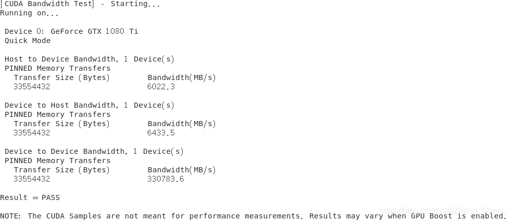
20241116（首马前夕）

• 伤痛确实未愈，忐忑不安，不知道能不能扛下来。

• 现在跑马已经一点热情都没有了，5分钟领完物就离开了，一点拍照的兴趣都没有。

• 我就知道老娘老爹过来准没好事，两个路痴，害我白走好多路找人，到中午得走了有十公里，脚都走疼了。然后中午吃完饭他们自己出去玩了，我已经累得不行，只想回去睡觉（AK他们下午也就去了趟明孝陵，根本走不动路，累死），一觉起来看到消息说晚饭让我解决，他们不回来吃饭了，我???

  • 不过晚上找到一家很好吃的面馆，叫劲来香牛肉面，物美价廉的一家西北面馆，羊肉串5块一串，买5送1，我直接炫了10串（留了两串给他们吃），比清真食堂的好吃，而且价格相仿（清真4块一串），外带一大碗牛腩刀削面，还能免费续面，还有免费的生大蒜跟牛骨汤喝，比中午那家抢钱的不知道强哪儿去了。

• PS：虽然但是，摆一张定妆照吧。跟诸位一路跑来的这三年，真的很开心。从五年前那个不欢而散的冬日，到三年前心灰意冷的夜晚，再到遇见诸位，让我这样的菜逼，也终于能练到如今的水平。筵席终散，与君共勉，来日相遇。
  

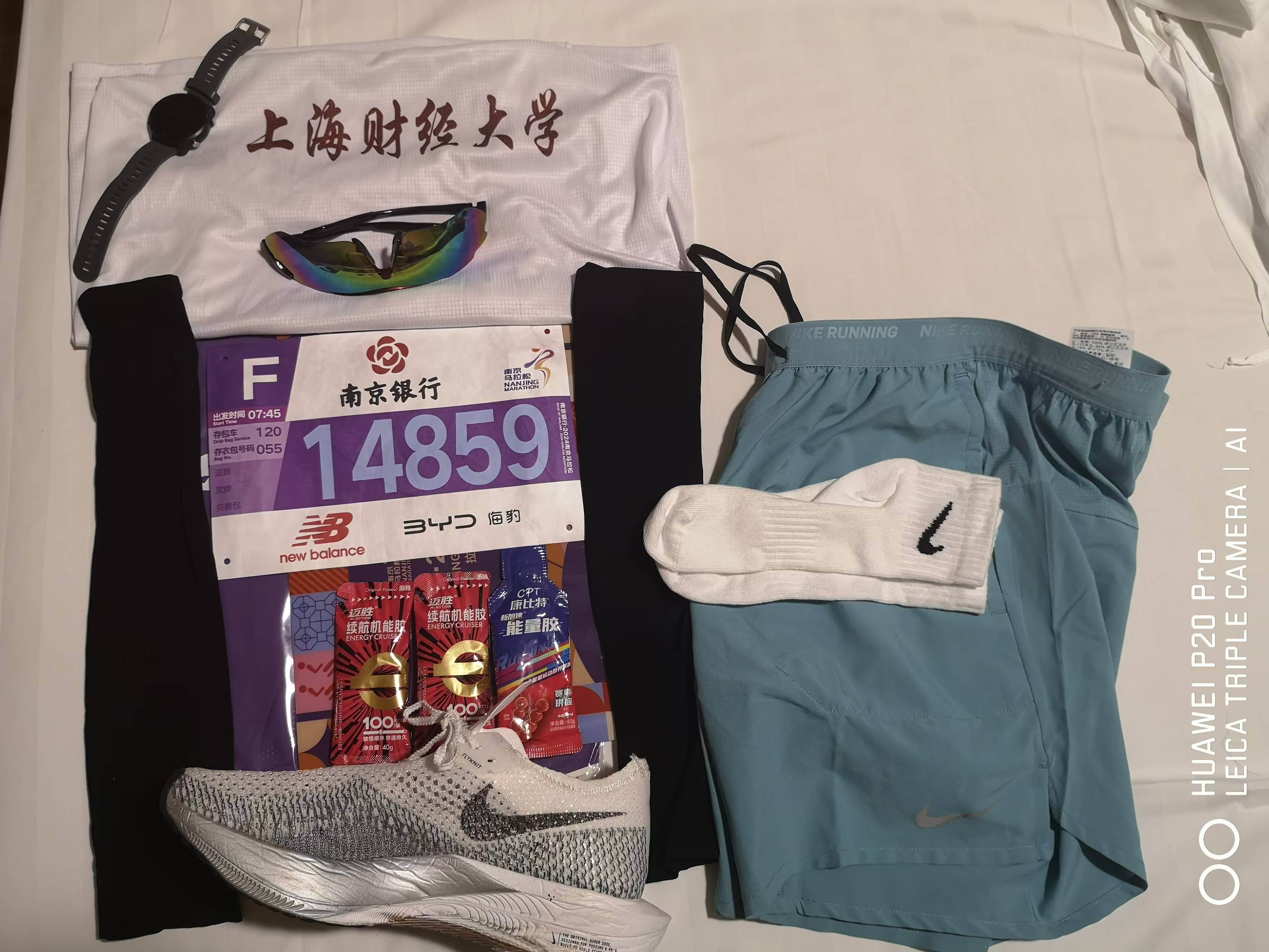
[性能测试] 03 单 4090 BERT、GPT2、T5 TFLOPS 测试及对比 3090TI

• 单位
  • K：10^3, 1e3, 千，thousand
  • M: 10^6, 1e6, 百万，million
  • G: 10^9, 1e9, 10亿，billion
  • T: 10^12, 1e12, 万亿，trillion
• TFLOPS, TFLOPs
  • TFLOPs：复数概念，多少个浮点数运算
  • TFLOPS：速度概念，每秒多少个浮点数运算
• transformer layer: BERT, GPT2, T5
  • (multi head attn) + ffn
  • multi head attn
    • 兼容 self attention 和 cross attention
    • 而 cross attn 只出现在 encoder + decoder 都有的情况
• 参考（李沐大神）
  • https://www.bilibili.com/video/BV1LT411F77M
  • https://github.com/mli/transformers-benchmarks/blob/main/micro_bench.ipynb

Mirco-Benchmarking for Transformers

This notebook benchmarks the most time consuming components in BERT, GPT-2 and T5 to help you understand its performance. Let’s first check our libraries and hardware. If your GPUs are recent models, please make sure your CUDA version is also recent, which may greatly affect the performance.

import torch
print('Pytorch version\t:', torch.__version__)
print('CUDA version\t:', torch.version.cuda)
print('GPU\t\t:',torch.cuda.get_device_name())
"""
Pytorch version	: 2.0.0+cu118
CUDA version	: 11.8
GPU		: NVIDIA GeForce RTX 4090
"""

Let’s first define a walltime method to benchmark Pytorch statements by at least 3 seconds.

import inspect
from collections import defaultdict
import pandas as pd
from torch.utils import benchmark 

pd.options.display.precision = 3

def var_dict(*args):
    callers_local_vars = inspect.currentframe().f_back.f_locals.items()
    return dict([(name, val) for name, val in callers_local_vars if val is arg][0] 
                for arg in args)

def walltime(stmt, arg_dict, duration=3):
    return benchmark.Timer(stmt=stmt, globals=arg_dict).blocked_autorange(
        min_run_time=duration).median

Last install huggingface from source code.

# 安装最新版本的 transformer（最新版本，源码安装）
from IPython.display import clear_output

!git clone git@github.com:huggingface/transformers.git
!cd transformers; pip install .

clear_output()
import transformers
print(transformers.__version__) # 4.30.0.dev0

Matrix Multiplication

Matrix multiplication is the most used operator in Transformers. Its performance is crucial. Let’s test the TFLOPS we can achieve on square matrices.

• TFLOPS：每s运行了多少次 tf（浮点运算），速度概念
  • TFLOPs：复数的概念
• $c_{n\cdot n}=a_{n\cdot n}\cdot b_{n\cdot n}$
  • 我们从结果（$c_{n\cdot n}$）出发，它的每一个位置（entry），都是由 $n$ 次乘法 + $n$ 次加法（准确地说是 $n-1$ 次加法）组成（矢量内积）
    • n+(n-1) = 2n-1 == 2n
  • $(n+n)\cdot n\cdot n=2n^3$
• 更高的 tflops：更大的矩阵乘法，float32 => float16
• float16
  • cuBLAS，使用 tensor cores；

# dict of dict
from tqdm import tqdm
matmul_tflops = defaultdict(lambda: {})
for n in tqdm([128, 512, 2*1024, 4*1024, 8*1024, 16*1024, 32*1024]):
    for dtype in (torch.float32, torch.float16):
        a = torch.randn(n, n, dtype=dtype).cuda()
        b = torch.randn(n, n, dtype=dtype).cuda()   
        t = walltime('a @ b', var_dict(a, b))
        matmul_tflops[f'n={n}'][dtype] = 2*n**3 / t / 1e12
        del a, b
        
pd.DataFrame(matmul_tflops)

n=128	n=512	n=2048	n=4096	n=8192	n=16384	n=32768
torch.float32	0.592	24.036	53.795	49.005	52.182	51.423	45.631
torch.float16	0.573	35.177	164.255	166.949	156.083	173.988	172.340

import matplotlib.pyplot as plt
xs = [128, 512, 2*1024, 4*1024, 8*1024, 16*1024, 32*1024]
plt.plot(xs, list(map(lambda x: matmul_tflops[f'n={x}'][torch.float32], xs)))
plt.plot(xs, list(map(lambda x: matmul_tflops[f'n={x}'][torch.float16], xs)))
plt.legend(['float32', 'float16'])

print('torch.float32', 53.795/42.056)
print('torch.float16', 173.988/81.314)
"""
torch.float32 1.279127829560586
torch.float16 2.1397053397938857
"""

You can see that the performance increases with the matrix size. If your GPU has Tensor Cores, you will see a big performance jump when switching from 32-bit floating points to 16-bit floating points.

Next you can find the theory TFLOPS of your GPU from Wikipedia, for example, Nvidia Tesla, Nvidia Quadro, RTX 40xx, RTX 30xx, and RTX 20xx. Here we list several cards, with their memory information.

Model	Memory (GB)	Memory Bandwidth (GB/sec)	FP32 TFLOPS	FP16 TFLOPS
A100	80	2039	19.5	312
V100	16	900	15.7	125
A6000	48	768	38	150
RTX 3090 TI	24	1008	40	160
RTX 4090	24	1008	82	330

If the best TFLOPS number you got is still far away from the theory TFLOPS of your GPU, the performance is likely bottlenecked by the memory bandwidth. To illustrate it, let’s benchmark a simple elemental-wise multiplication to show both its TFLOPS with memory bandwidth.

• 深度学习中的按元素（element wise）运算：
  • 一个layer的输出，经过 activate function；
  • 权重的更新；

vector = defaultdict(lambda: {})
# *4
for n in [1024*64, 1024*256, 1024*1024, 1024*1024*4, 1024*1024*16, 1024*1024*64]:
    a = torch.randn(n).cuda()
    t = walltime('a * 1.2', var_dict(a))
    vector[n]['TFLOPS'] = n / t / 1e12
    # float32: 4 Byte;
    # 读写：两个操作；
    vector[n]['GB/s'] = (4*2) * n / t / 1e9
    
pd.DataFrame(vector)

	    65536	262144	1048576	4194304	16777216	67108864
TFLOPS	0.009	0.043	0.173	0.472	0.115	0.115
GB/s	70.541	343.917	1385.415	3777.138	920.339	921.202

You can see that even for large vectors, the TFLOPS is far far way from GPU peak performance, while the bandwidth may be quite close to its theoretical number.

The matrix multiplication performance is a main topic in HPC. There are a large number of research papers. Unfortunately the backend library, cuBLAS, is not open sourced. You may check cutlass, which claimed similar performance as cuBLAS, for some implementation details.

BERT Layer

The main body of a Transformer model is a stacking of Transformer blocks. Let’s benchmark the performance of a single block. In BERT, it is often called a BERT layer. Let’s construct one such layer from the BERT large model. We use 16-bit floating points for better performance.

from transformers import AutoConfig, BertLayer

config = AutoConfig.from_pretrained("bert-large-uncased")
layer = BertLayer(config).half().cuda()
# multihead attention: 64*16
print(config.hidden_size) # 1024

Then define a function to benchmark both forward and forward with backward performance using different sequence lengths and batch sizes.

• input_shape: (b, s, h)
• ffn：
  • 两层 mlp，h=>4h=>h
    • h->4h
      • (b, h)*(h, 4h) => (b, 4h)
      • (b*4h)(2*h) == 8*b*h*h
    • 4h->h
      • (b, 4h)*(4h, h) => (b, h)
      • (b*h)*(2*4*h) == 8*b*h*h
    • 16*b*h*h
    • 16*b*s*h*h
• attn：假如有 n 个头，每个头的维度：h/n（Q，K，V）
  • 三步
    • 第一步先做投影，
      • Q: (s, h) * (h, h/n) ==> (s, h/n)
        • s*(h/n)*(2h)
      • K: (s, h) * (h, h/n) ==> (s, h/n)
        • s*(h/n)*(2h)
      • V: (s, h) * (h, h/n) ==> (s, h/n)
        • s*(h/n)*(2h)
      • s*(h/n)*(2h)*3 = 6*(h*h/n)*s
    • 再计算 attn_score: (Q*K^T)*V
      • (s, h/n) * (h/n, s) => (s, s)
        • s*s*(2h/n)
      • (s,s)*(s, h/n) => (s, h/n)
        • (s*h/n)*(2s)
      • s*s*(2h/n) + (s*h/n)*(2s) = 4*(h/n)*s*s
    • n个(h/n) concat 为 h，做一次投影 (s, h) => (s, h)
      • (6*(h*h/n)*s + 4*(h/n)*s*s) * n = 6*s*h*h + 4*h*s*s
      • (s, h) * (h, h) => (s, h)
        • s*h*(2*h) = 2*s*h*h
    • 6*s*h*h + 4*h*s*s + 2*s*h*h = 8*s*h*h + 4*h*s*s

def layer_benchmark(layer, hidden_size, seq_lens, batch_sizes, cross_attention=False):
    h = hidden_size
    results = defaultdict(lambda: {})    
    encoder_state = 'encoder_hidden_states=X' if cross_attention else ''
    for s in seq_lens:
        for b in batch_sizes:            
            ffn = 16*b*s*h*h / 1e12  # TFLOPs for the Feed-Forward Network
            atten = (4*b*h*s*s + 8*b*s*h*h) / 1e12  # TFLOPs for attention            
            forward = ffn + (2 if cross_attention else 1) * atten
            
            X = torch.randn(b, s, h).half().cuda()
            results[f'batch={b}'][f'fwd seq_len={s}'] = forward / walltime(
                f'layer(X, {encoder_state})', var_dict(layer, X))
            results[f'batch={b}'][f'fwd+bwd seq_len={s}'] = 3 * forward / walltime(
                f'layer(X, {encoder_state})[0].sum().backward()', var_dict(layer, X))            
    return pd.DataFrame(results)

In BERT pre-training, we often train with a sequence of 128 (stage 1) or 512 (stage 2). Let’s test its performance.

layer_benchmark(layer, config.hidden_size, [128, 512], [2, 4, 8, 16, 32, 64, 128])

	 batch=2	batch=4	batch=8	batch=16	batch=32	batch=64	batch=128
fwd seq_len=128	11.511	13.321	45.993	53.099	107.170	110.394	97.590
fwd+bwd seq_len=128	3.129	6.341	12.523	25.068	49.649	99.831	102.060
fwd seq_len=512	29.852	82.675	76.396	73.583	71.270	68.964	69.280
fwd+bwd seq_len=512	13.490	26.978	53.157	80.533	76.346	78.427	78.398

110.394/56.488 ⇒ 1.9542911768871265

No surprise that a large batch size helps. But the best number is below the matrix multiplication TFLOPS. Let’s find why.

We first benchmark the first dense layer in the Feed-Forward Network (FFN) in the layer.

# ffn 中的其中一层 mlp, h=>4h
layer.intermediate.dense # Linear(in_features=1024, out_features=4096, bias=True)

h, b, s = config.hidden_size, 64, 128
X = torch.randn(b, s, h).half().cuda()

'Dense layer TFLOPS: %.3f' % (8*b*s*h*h / 1e12 / walltime(    
    'layer.intermediate.dense(X)', var_dict(layer, X))) # 'Dense layer TFLOPS: 160.980'

The number is pretty good. Then run this dense layer with the GeLU activation.

# ffn 中的其中一层 mlp
layer.intermediate
'Dense+Activation TFLOPS: %.3f' % (8*b*s*h*h / 1e12 / walltime(
    'layer.intermediate(X)', var_dict(layer, X))) # 'Dense+Activation TFLOPS: 126.240'

Even the activation function has a ignorable complexity, it brings down the TFLOPS. We pointed out the reason before, the elemental-wise operation of the activation function is bounded by the memory bandwidth.

Now test the whole FFN.

ffn = 16*b*s*h*h / 1e12
'FFN TFLOPS: %.3f'%(ffn / walltime(
    'layer.output(layer.intermediate(X),X)', var_dict(layer, X))) # 'FFN TFLOPS: 135.765'

The other part in the BERT layer is the multi-head self-attention.

att = (4*b*h*s*s + 8*b*s*h*h) / 1e12
'Attention TFLOPS: %.3f'%(
    att / walltime('layer.attention(X)', var_dict(layer, X))) # 'Attention TFLOPS: 81.950'

Even though the main computation part of the attention block is still matrix multiplication, it has more memory bounded operators compared to FFN. So you see a lower TFLOPS.

att / ffn ⇒ 0.53125

The ratio of complexity between attention and FFN depends on the BERT configuration. The overall performance is a weighted sum between the FLOPS of these two components.

GPT-2网络块

Next let’s evaluate gpt2-medium, which has a similar architecture has bert-large, i.e. 24 layers with a 1024 hidden size. GPT2 is trained with a 1024 sequence length.

from transformers.models.gpt2.modeling_gpt2 import GPT2Block

config = AutoConfig.from_pretrained("gpt2-medium")
layer = GPT2Block(config, layer_idx=0).half().cuda()
layer_benchmark(layer, config.n_embd, [512, 1024], [2, 4, 8, 16, 32, 64])

batch=2	batch=4	batch=8	batch=16	batch=32	batch=64
fwd seq_len=512	25.072	49.734	56.900	49.412	48.346	47.935
fwd+bwd seq_len=512	12.614	25.118	49.785	54.885	53.958	54.169
fwd seq_len=1024	44.208	43.629	39.372	38.740	38.568	38.427
fwd+bwd seq_len=1024	27.067	44.980	44.579	43.975	44.094	44.113

56.900/36.595 ⇒ 1.5548572209318212

You can see that, despite GPT-2 and BERT has the same complexity, GPT-2 has slightly worse TFLOPS when using the same batch size and sequence length. Also using a larger sequence length 1024 further harms the performance.

T5 Layer

T5 has both encoder and decoder, let’s first benchmark the decoder, whose performance is similar to BERT.

from transformers.models.t5.modeling_t5 import T5Block

config = AutoConfig.from_pretrained("t5-large")
config.use_cache = False
config.is_decoder = False
config.is_encoder_decoder = False

encoder = T5Block(config).half().cuda()
layer_benchmark(encoder, config.d_model, [512], [2, 4, 8, 16, 32, 64, 128])

	batch=2	batch=4	batch=8	batch=16	batch=32	batch=64	batch=128
fwd seq_len=512	19.052	50.302	47.720	45.154	43.313	41.821	41.524
fwd+bwd seq_len=512	10.798	21.681	41.511	52.429	49.602	49.603	49.468

The decoder has an additional cross attention, which increases the time complexity and also hurts TFLOPS.

config.is_decoder = True
decoder = T5Block(config).half().cuda()
layer_benchmark(decoder, config.d_model, [512], [2, 4, 8, 16, 32, 64, 128], cross_attention=True)

	batch=2	batch=4	batch=8	batch=16	batch=32	batch=64	batch=128
fwd seq_len=512	29.277	40.767	38.341	36.989	35.458	34.330	34.084
fwd+bwd seq_len=512	9.257	18.400	36.701	42.897	40.398	40.718	40.643

总之，为了实现Transformer层的最佳性能，需要使用快速的数据类型（比如bf16）和大的batchsize。有时候为了更好的性能，可能需要重写代码。例如，将原先代码的多个kernel融合为一个kernel。

---

20241117（完篇）

一：楔子

我们总说，首马对于跑者的意义，就像高中老师强调高考对于人生的意义一样。其实也就那么一回事，对吧？只是，总是要经历一回才行。

不同于上半年创造PB的扬州半马，那时的我具备有史以来最硬的实力，长达一个多月的规律饮食作息调整得到极佳的精神状态，加上主场作战的充分准备，比赛日极好的天气的加成，真是占尽天时地利人和。

然而，首马的赛前几乎是另一个极端，长期的熬夜的不规律作息，从高百那周开始就一直没完全康复的感冒，好在饮食还算比较健康。唯一能拿得出手的可能就是连续五个月的200K左右的月跑量，月均配410-420，看起来还算高质量的训练，可其中缺少了必要的长距离拉练——我根本就没有任何把握能跑完全马。

最雪上加霜的是，赛前十日遭遇右足弓伤痛，一直到今早走路都明显能感觉得到疼痛。我不知道这种疼痛到底会在长达42公里的赛程中，发展到何种程度。

凌晨，窗外雨疏风骤，气温骤降。尽管很早就熄了灯，但直到将近两点才能入睡，并不是因为比赛而兴奋，只是感性于昨晚发生的一些事情。

真的能用这副身体扛下三小时的全马吗？

——混沌之间，为懦夫，抑或莽夫？

---

二：风暴

其实当懦夫也没什么不好的，对吧。

我选择了缓和Vaporfly3，而非激进的160X3.0Pro作为比赛鞋。因为我决定用全程后跟跑而非前掌跑，这样对足弓的压迫小，虽然慢但安全些。

早上出门前我只吃了一包干拌方便面和一小块面包，水都只喝了小半杯，想着到起点会有水和香蕉的补给。

显然，我是想多了，奥体中心根本什么都没有。

更糟糕的是，存包的时候，我忘记把包里的能量胶和盐丸取出，以至于整场比赛期间，我只能通过喝水进行补给，一根胶都没吃到（后来AK说这就是我后程大崩的原因，不补给肯定是不行的）。

径直检录进入F区，我连厕所都没去上（当然一部分原因是排队的人太多，我也懒得去排，比赛途中我不止一次想停下来去上厕所，但实际上全程我没有停下任何一次）。

拉倒，反正已经衰成这样了，再衰一点也没差了。

---

三：摆烂？拼命？

上午第二枪7点45分发枪，身处F区的我直到7点52分才抵达起跑线，此时已经过去了7分多钟，前方早已是人山人海。要知道上半年扬州半马我也不过只花了3分钟就到达起点，但即便如此我前10KM都在努力突围，在8KM处才追上A区的130兔子。

还是摆吧，起跑后的5K，我都不太想去刻意提速见缝插针，跟着几个的小团体慢悠悠的晃着，这样真的好舒服，身体很轻很轻（得益于赛前真的没吃啥东西），心率也特别低。

其实本来也不太能跑得开，加上雨天场地潮湿，我也不太想全马一上来就拼刺刀，毕竟跟半马还是不一样的。

5K之后人群疏松了许多，转折点在于11K，我遇到了两个南大定向越野队的队员，他俩基本以350-355在巡航，我突然有了些精神，不如陪他俩耍耍，跟了2K之后我越来越兴奋，但是我很清楚自己不可能以这种配速跑完全马，还是理智地放弃了。然而，兴奋的势头不是那么容易衰减的，这段变速让我觉得自己还是可以去拼一拼的，要把之前失去的时间追回来也未尝不可能。

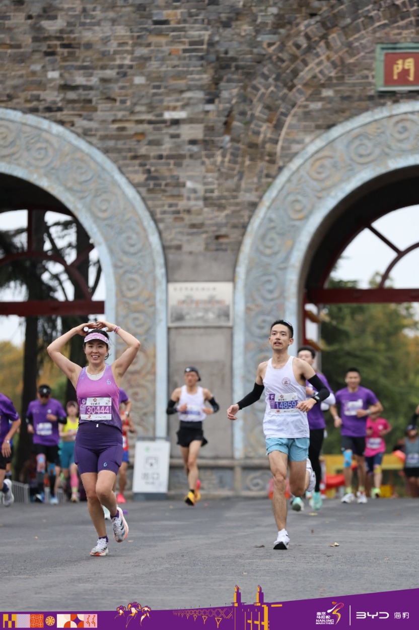
事实上，半程经过玄武门计时点👆，用时为1小时33分，这已经不算慢了，尽管大概率不能破三，但是想跑进310还是很有机会的。最重要的是，经过玄武门时我感觉自己余力尚足，当时就已经确信自己肯定是能顺利完赛了。

我的自信在接下来的分段得到了验证，20-25K依然保持了相对较高的配速，直到30K结束，每公里的用时都没有掉出4分30秒👇

---

四：写在30KM后

然而，全马从30K，才刚刚开始。

从结果来看，我从第31K就开始出现了明显的掉速，但是这是我当时保守的策略，一方面，我有算过，就算放到440的均配跑完最后12K多，也能顺利跑进310，至于到底是30X，这已经不关键了，反正是破不了三，X是多少没有任何区别；另一方面，是对全马的敬畏，我清楚30K是一个转折点，尽管当时体感依然保有余力，但我觉得适当放缓一些是明智的。

真正的撞墙感来自33-34K这段，这段刚好是江边的偏北风呼啸，逆风上坡段，说实话这种情况发生在30K之后是非常致命的，大量的人在这段区间开始停下行走，此时我也已经感觉脚后跟非常疼了，连续两个半小时的后跟跑已经让脚后跟出现如同尖刺般的疼痛，每一步都极其艰难，不同于30K之后主动的掉速，这里我已经感觉越来越维持不了节奏，只能任由自己掉速。

此时，赛场出现关键的变数，我发现一位身着南师大背心的女生超过了我。我很轻地说了一声南师大，她大概也看到了我背心上的学校名，对我挥手示意，这特么我能忍？直接抬腿就把她超了，然后在下一个补给点她又反超了回来。

虽然跑不赢女生很丢人，但我确实强弩之末，已经跑不动了，想想大丈夫能屈能伸，要不跟着小香风也不错，这也是35-37K这关键的3KM又能重回4分半配速的原因。只可惜到38K我真的是跟不住她了，在我即将掉队的时候，我追上问了一下她是从哪个区出发的，我幻想她可能是D区E区，甚至是第一枪出发的，结果她告诉我她是F区出发，今天也是首马，我???，只能感叹一句你真的太强了（目测她肯定是跑进310了，这个已经是超国家一级的水平了）。

轻松自信的笑容跟我的痛苦面具形成鲜明对比（真不忍直视自己的脸了），我真的太菜了👇

---

五：行百里半九十

被南师大的小姐姐拉爆之后，我整个人的心态、心率、大腿、小腿、脚已经全部都崩盘了。

• 心态崩盘自不必说，这已经是多少次吃女生的辣堡了？讽刺地是，就在我被拉爆后，一位老哥从后面高歌猛进，看着一帮走走停停的人说，35K之后才是疯狂收割，贱笑得让我想上去抽他，可惜我追不上他。

• 心率已经几乎稳定保持在180bpm以上，有一段我试着想从六分配提到五分半的配速，心率直接飙到190bpm。

• 大腿小腿完全不是自己的腿，每迈一步都是在和脚后跟疼痛做抗争。

可是我不能停下，我想到大家给我发的消息，只要跑着就好，求求了，慢就慢一些，至少凭借意志维持一个跑步的动作不难吧，也就最后三四公里了。

我从来没有觉得一公里有这么长过，最慢的第40公里我用了整整5分58秒，我以前嘲讽SXY说六分配以外不就是走路吗？现在看来六分配也不是很慢了。

我迫切地想要停下来走，身边也有大批停下走路的人，但是我知道以目前这种疼痛感，只要我停下来，就再也跑不起来了。

终于，40KM计时点用时超过了3个小时，全程均配掉出了4分30秒。

已经不可能跑进310了，退而求其次，至少315吧。一定不能停下来走，我脑中只想着这一点，否则连315都做不到了。

---

六：终点

3小时14分10秒，这是我最终交出的首马答卷。事实上，今天的南马是极好的天气，有超过2200人破三，几乎每10人中就有一名破三选手。

到终点后，我险些就要倒下，腿已经完全站不住了，必须要扶着栏杆才能艰难前行。我走了好久才找到自己的存包，拿到手机报了声平安。

首马314，尽管没有达到预期，但的确也不算很差了，胡哥首马326，AX首马324，嘉伟首马259，AK首马253，安迪两次全马都没跑进345。

而且严格来说我到38K才算是彻底跑崩，这已经高出我的预期了，我原以为半程之后可能就会崩。

DGL说把她的好运借给我，我还真就顺利跑完全程了，足弓的疼痛没有发展到不可调和的地步，现在的疼的位置只是脚踝一圈的前侧，那里疼只是因为全程后跟跑造成的持续压迫，应该很快就会康复。

伤痛竟然没有复发，有时候是得相信一些玄学的，得道多助，失道寡助。

---

后记

这会是完结吗？

筵席终散，跑步也是一样的。

SXY说还会有很多场马拉松会去跑，可是我真的一点儿都不想再去跑全马了。

就这么… 可还是好想能破三。今天刘守征也破三了，我还是不行。

不知道，也许睡一觉好了。

END@Yangzhou