支持向量机学习之3-SVR（回归）

ϵ−SVR

SVR回归中，基本思路和SVM中是一样的，在 ϵ−SVR [Vapnic,1995] 需要解决如下的优化问题。 

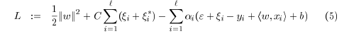
min  12||w||2+C∑i=1l(ξi+ξ∗i)

s.t.  ⎧⎩⎨⎪⎪⎪⎪yi−(wTxi+b)<ϵ+ξi(wTxi+b)−yi<ϵ+ξ∗iξi,ξ∗i≥0

细心的读者可能已经发现了与 C−SVM 中的具有相似的地方，但又不太一样，那么如何理解上述公式呢？ 
假设我们的训练数据集是 {(x1,y1),(x2,y2),...(xn,yl)}  
我们的目标是找到一个函数，比如线性函数 f(x)=wTx+b ,使得 
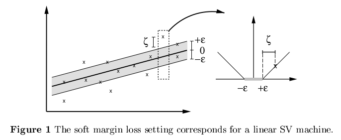
如果数据离回归函数的偏差 |yi−wTx−b|<ϵ| (下图非色区域）,我们是能接受的，不需要付出任何代价（即不需要在代价函数中体现）。我们只关注偏差大于 ϵ 的代价。举个例子来说，就好比我们在换外币时，我们并不关注少量 ϵ 损失，这部分损失是汇率引起的合理损失。 
所以约束条件是保证更多多的数据点都在灰色范围内（拟合最佳的线性回归函数，使得更多的点落在我们接受的精度范围内），即 |yi−wTx−b|<ϵ| 。但是我们发现，还是会有一部分点，偏差比较大，落在灰色区域之外，所以类似SVM中使用的方法，引入松弛因子，采取软边界的方法，而且上下采取不同的松弛因子 ξi,ξ∗i≥0 ，这样就不难得出约束条件为： 

s.t.  ⎧⎩⎨⎪⎪⎪⎪yi−(wTxi+b)<ϵ+ξi(wTxi+b)−yi<ϵ+ξ∗iξi,ξ∗i≥0

 
如同SVM中一样的，在多数情况下转换为对偶问题更容易计算。同时还可以计算出 w 和 b ，直接看文献1吧。 
 
 
 
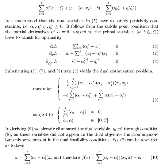
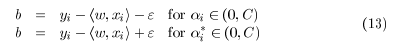
详细推导过程看文献1。

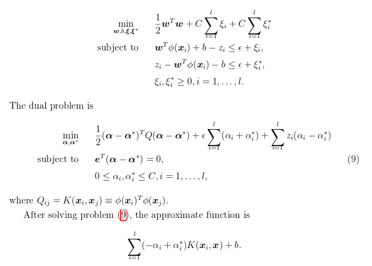
使用核函数的 ϵ−SVR

文献2 

ν−SVR

 
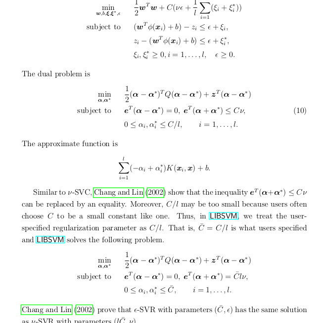
Chang and Lin (2002) prove that ϵ -SVR with parameters  (C¯¯¯̄ ,ϵ) has the same solution as  ν -SVR with parameters (lC¯¯¯̄ ,ν) . 
其实两种SVR在满足一定条件下，具有相同的解。

优缺点分析

Scikit代码

#-*-coding:utf-8-*- 
import numpy as np  
from sklearn.svm import SVR  
import matplotlib.pyplot as plt  

###############################################################################  
# Generate sample data  
X = np.sort(5 * np.random.rand(40, 1), axis=0)  #产生40组数据，每组一个数据，axis=0决定按列排列，=1表示行排列  
y = np.sin(X).ravel()   #np.sin()输出的是列，和X对应，ravel表示转换成行  

###############################################################################  
# Add noise to targets  
y[::5] += 3 * (0.5 - np.random.rand(8))  

###############################################################################  
# Fit regression model  
svr_rbf10 = SVR(kernel='rbf',C=100, gamma=10.0)  
svr_rbf1 = SVR(kernel='rbf', C=100, gamma=0.1)  
svr_rbf1 = SVR(kernel='rbf', C=100, gamma=0.1)  
#svr_lin = SVR(kernel='linear', C=1e3)  
#svr_poly = SVR(kernel='poly', C=1e3, degree=3)  
y_rbf10 = svr_rbf10.fit(X, y).predict(X)  
y_rbf1 = svr_rbf1.fit(X, y).predict(X) 
#y_lin = svr_lin.fit(X, y).predict(X)  
#y_poly = svr_poly.fit(X, y).predict(X)  

###############################################################################  
# look at the results  
lw = 2 #line width  
plt.scatter(X, y, color='darkorange', label='data')  
plt.hold('on')  
plt.plot(X, y_rbf10, color='navy', lw=lw, label='RBF gamma=10.0')  
plt.plot(X, y_rbf1, color='c', lw=lw, label='RBF gamma=1.0')  
#plt.plot(X, y_lin, color='c', lw=lw, label='Linear model')  
#plt.plot(X, y_poly, color='cornflowerblue', lw=lw, label='Polynomial model')  
plt.xlabel('data')  
plt.ylabel('target')  
plt.title('Support Vector Regression')  
plt.legend()  
plt.show()
 
 
1
2
3
4
5
6
7
8
9
10
11
12
13
14
15
16
17
18
19
20
21
22
23
24
25
26
27
28
29
30
31
32
33
34
35
36
37
38
39
40

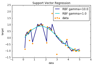
RBF不同参数： 
 
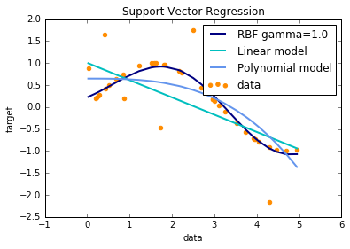
不同核函数：