【机器学习】随机森林

• 🍨 本文为🔗365天深度学习训练营 中的学习记录博客
• 🍖 原作者：K同学啊

一、随机森林定义

随机森林（Random Forest, RF）是一种由 决策树 构成的 集成算法 ，采用的是 Bagging 方法，他在很多情况下都能有不错的表现。如下表。

二、数据读取

import pandas as pd
import numpy as np
import seaborn as sns
import matplotlib.pyplot as plt
from sklearn.preprocessing import LabelEncoder
from sklearn.model_selection import train_test_split
from sklearn.ensemble import RandomForestClassifier
from sklearn.metrics import classification_report

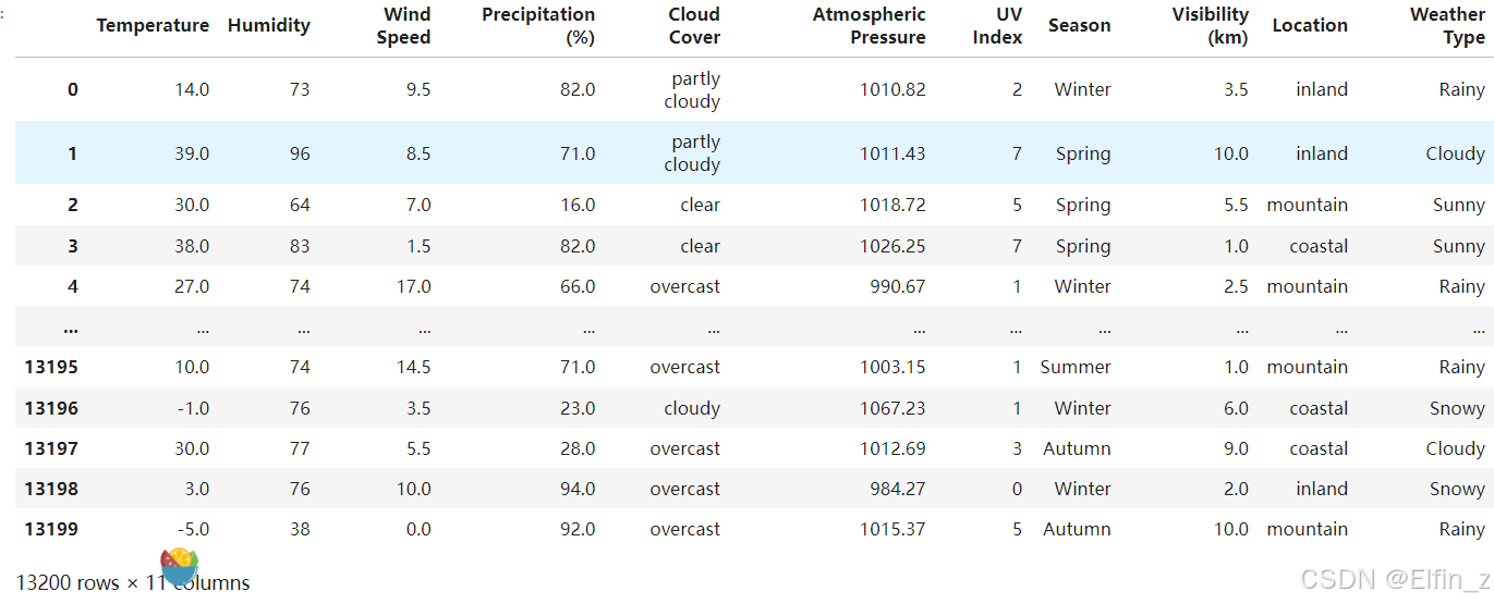
data = pd.read_csv('D:/Personal Data/Learning Data/DL Learning Data/weather_classification_data.csv')
data

三、数据检查与预处理

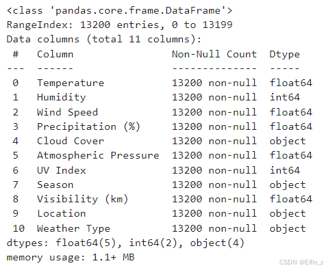
# 查看数据信息
data.info()

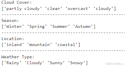
# 查看分类特征的唯一值
characteristic = ['Cloud Cover','Season','Location','Weather Type']
for i in characteristic:
    print(f'{i}:')
    print(data[i].unique())
    print('-'*50)

feature_map = {
    'Temperature': '温度',
    'Humidity': '湿度百分比',
    'Wind Speed': '风速',
    'Precipitation (%)': '降水量百分比',
    'Atmospheric Pressure': '大气压力',
    'UV Index': '紫外线指数',
    'Visibility (km)': '能见度'
}
plt.figure(figsize=(15, 10))

for i, (col, col_name) in enumerate(feature_map.items(), 1):
    plt.subplot(2, 4, i)
    sns.boxplot(y=data[col])
    plt.title(f'{col_name}的箱线图', fontsize=14)
    plt.ylabel('数值', fontsize=12)
    plt.grid(axis='y', linestyle='--', alpha=0.7)

plt.tight_layout()
plt.show()

print(f"温度超过60°C的数据量：{data[data['Temperature'] > 60].shape[0]}，占比{round(data[data['Temperature'] > 60].shape[0] / data.shape[0] * 100,2)}%。")
print(f"湿度百分比超过100%的数据量：{data[data['Humidity'] > 100].shape[0]}，占比{round(data[data['Humidity'] > 100].shape[0] / data.shape[0] * 100,2)}%。")
print(f"降雨量百分比超过100%的数据量：{data[data['Precipitation (%)'] > 100].shape[0]}，占比{round(data[data['Precipitation (%)'] > 100].shape[0] / data.shape[0] * 100,2)}%。")

print("删前的数据shape：", data.shape)
data = data[(data['Temperature'] <= 60) & (data['Humidity'] <= 100) & (data['Precipitation (%)'] <= 100)]
print("删后的数据shape：", data.shape)

删前的数据shape： (13200, 11)
删后的数据shape： (12360, 11)

四、数据分析

data.describe(include='all')

plt.figure(figsize=(20, 15))
plt.subplot(3, 4, 1)
sns.histplot(data['Temperature'], kde=True,bins=20)
plt.title('温度分布')
plt.xlabel('温度')
plt.ylabel('频数')

plt.subplot(3, 4, 2)
sns.boxplot(y=data['Humidity'])
plt.title('湿度百分比箱线图')
plt.ylabel('湿度百分比')

plt.subplot(3, 4, 3)
sns.histplot(data['Wind Speed'], kde=True,bins=20)
plt.title('风速分布')
plt.xlabel('风速（km/h）')
plt.ylabel('频数')

plt.subplot(3, 4, 4)
sns.boxplot(y=data['Precipitation (%)'])
plt.title('降雨量百分比箱线图')
plt.ylabel('降雨量百分比')

plt.subplot(3, 4, 5)
sns.countplot(x='Cloud Cover', data=data)
plt.title('云量 (描述)分布')
plt.xlabel('云量 (描述)')
plt.ylabel('频数')

plt.subplot(3, 4, 6)
sns.histplot(data['Atmospheric Pressure'], kde=True,bins=10)
plt.title('大气压分布')
plt.xlabel('气压 (hPa)')
plt.ylabel('频数')

plt.subplot(3, 4, 7)
sns.histplot(data['UV Index'], kde=True,bins=14)
plt.title('紫外线等级分布')
plt.xlabel('紫外线指数')
plt.ylabel('频数')

plt.subplot(3, 4, 8)
Season_counts = data['Season'].value_counts()
plt.pie(Season_counts, labels=Season_counts.index, autopct='%1.1f%%', startangle=140)
plt.title('季节分布')

plt.subplot(3, 4, 9)
sns.histplot(data['Visibility (km)'], kde=True,bins=10)
plt.title('能见度分布')
plt.xlabel('能见度（Km）')
plt.ylabel('频数')

plt.subplot(3, 4, 10)
sns.countplot(x='Location', data=data)
plt.title('地点分布')
plt.xlabel('地点')
plt.ylabel('频数')

plt.subplot(3, 4, (11,12))
sns.countplot(x='Weather Type', data=data)
plt.title('天气类型分布')
plt.xlabel('天气类型')
plt.ylabel('频数')

plt.tight_layout()
plt.show()

五、随机森林

new_data = data.copy()
label_encoders = {}
categorical_features = ['Cloud Cover', 'Season', 'Location', 'Weather Type']
for feature in categorical_features:
    le = LabelEncoder()
    new_data[feature] = le.fit_transform(data[feature])
    label_encoders[feature] = le

for feature in categorical_features:
    print(f"'{feature}'特征的对应关系：")
    for index, class_ in enumerate(label_encoders[feature].classes_):
        print(f"  {index}: {class_}")

# 构建x，y
x = new_data.drop(['Weather Type'],axis=1)
y = new_data['Weather Type']

# 划分数据集
x_train,x_test,y_train,y_test = train_test_split(x,y,
                                                 test_size=0.3,
                                                 random_state=15) 

# 构建随机森林模型
rf_clf = RandomForestClassifier(random_state=15)
rf_clf.fit(x_train, y_train)

# 使用随机森林进行预测
y_pred_rf = rf_clf.predict(x_test)
class_report_rf = classification_report(y_test, y_pred_rf)
print(class_report_rf)

六、结果分析

feature_importances = rf_clf.feature_importances_
features_rf = pd.DataFrame({'特征': x.columns, '重要度': feature_importances})
features_rf.sort_values(by='重要度', ascending=False, inplace=True)
plt.figure(figsize=(10, 8))
sns.barplot(x='重要度', y='特征', data=features_rf)
plt.xlabel('重要度')
plt.ylabel('特征')
plt.title('随机森林特征图')
plt.show()

随机森林模型的预测准确率很高，并且通过特征度分析，发现影响模型的主要因素有：温度、湿度、紫外线指数、能见度、大气压力。

七、总结

数据预处理对于任何模型而言都是至关重要的。其中包含了对空值的处理、去重、去除噪声数据等。