小白带你深度学习DAY2

代码说明

1. 数据预处理：

   • 使用Normalize将像素值从[0,1]归一化到[-1,1]

   • 自动下载CIFAR-10数据集（约163MB）

2. 模型结构：

   包含两个卷积层和两个池化层，直观展示特征图尺寸变化

3. 可视化内容：

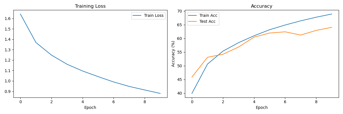
   • 训练损失曲线（左图）

   • 训练集和测试集准确率曲线（右图）

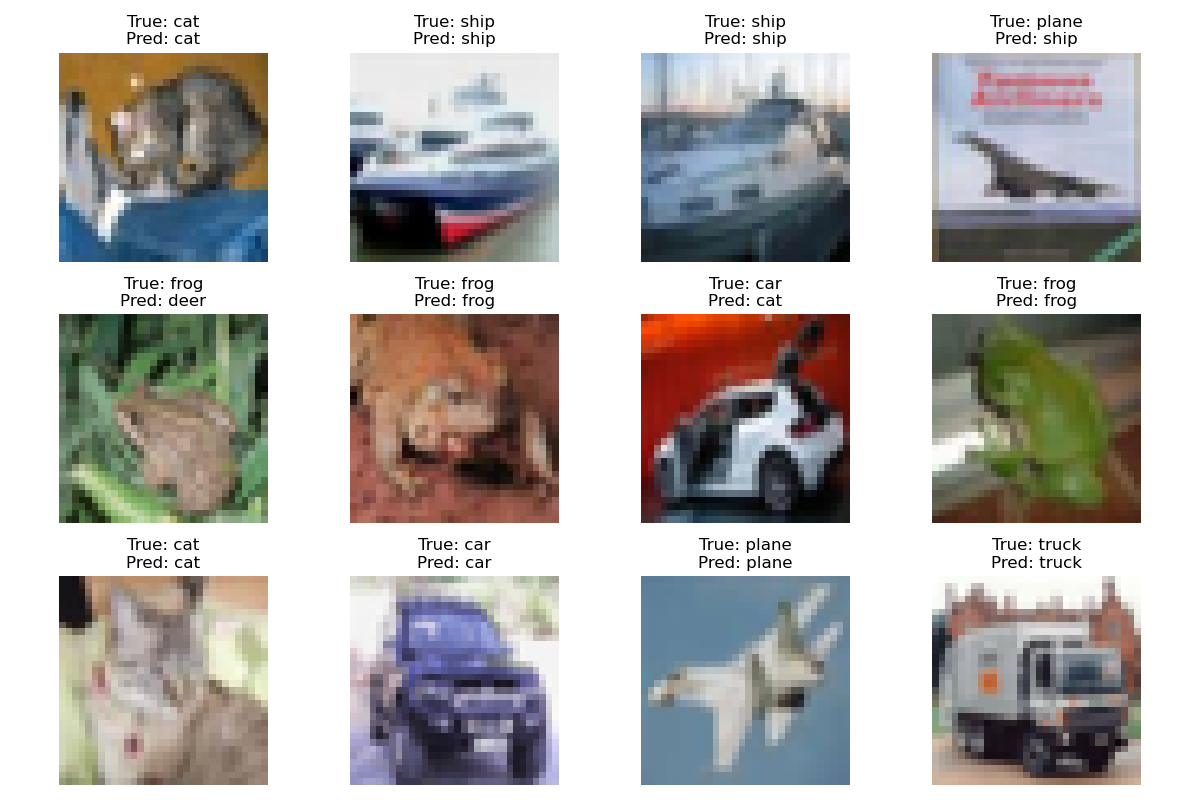
   • 12个测试样本的预测结果（显示真实标签与预测标签）

     

运行准备

1. 安装：

   pip install torch torchvision matplotlib

2. 运行：

   • 首次运行会自动下载CIFAR-10数据集到./data目录

   • 如果使用GPU训练，将自动检测并启用

   • 训练约10分钟后（在CPU上）可看到完整结果

3. 输出：

   • 训练过程中会打印每个epoch的损失和准确率

   • 最终显示两张图表和预测示例图

   • 测试准确率约60%-65%（可通过增加epoch提升）

import torch
import torchvision
import torch.nn as nn
import torch.optim as optim
import matplotlib.pyplot as plt
import numpy as np
import os
os.environ['KMP_DUPLICATE_LIB_OK']='True'

# 超参数设置
BATCH_SIZE = 64
EPOCHS = 10
LR = 0.001

device = torch.device("cuda" if torch.cuda.is_available() else "cpu")

# -------------------- 数据加载 --------------------
transform = torchvision.transforms.Compose([
    torchvision.transforms.ToTensor(),
    torchvision.transforms.Normalize((0.5, 0.5, 0.5), (0.5, 0.5, 0.5))
])

train_dataset = torchvision.datasets.CIFAR10(
    root='./data', train=True, download=True, transform=transform)
test_dataset = torchvision.datasets.CIFAR10(
    root='./data', train=False, download=True, transform=transform)

train_loader = torch.utils.data.DataLoader(
    train_dataset, batch_size=BATCH_SIZE, shuffle=True)
test_loader = torch.utils.data.DataLoader(
    test_dataset, batch_size=BATCH_SIZE, shuffle=False)

classes = ('plane', 'car', 'bird', 'cat', 'deer',
           'dog', 'frog', 'horse', 'ship', 'truck')


# -------------------- 修正后的模型 --------------------
class SimpleCNN(nn.Module):
    def __init__(self):
        super(SimpleCNN, self).__init__()
        self.conv_layers = nn.Sequential(
            nn.Conv2d(3, 6, kernel_size=5),
            nn.ReLU(),
            nn.MaxPool2d(2, stride=2),
            nn.Conv2d(6, 16, kernel_size=5),
            nn.ReLU(),
            nn.MaxPool2d(2, stride=2)
        )
        self.fc_layers = nn.Sequential(
            nn.Linear(16 * 5 * 5, 120),
            nn.ReLU(),
            nn.Linear(120, 84),
            nn.ReLU(),
            nn.Linear(84, 10)
        )  # 修正点1：补全括号

    def forward(self, x):
        x = self.conv_layers(x)
        x = x.view(x.size(0), -1)  # 修正点2：正确写法
        x = self.fc_layers(x)
        return x


model = SimpleCNN().to(device)

# -------------------- 训练部分保持不变 --------------------
criterion = nn.CrossEntropyLoss()
optimizer = optim.Adam(model.parameters(), lr=LR)

train_loss_history = []
train_acc_history = []
test_acc_history = []

for epoch in range(EPOCHS):
    model.train()
    running_loss = 0.0
    correct = 0
    total = 0

    for images, labels in train_loader:
        images, labels = images.to(device), labels.to(device)
        outputs = model(images)
        loss = criterion(outputs, labels)
        optimizer.zero_grad()
        loss.backward()
        optimizer.step()

        running_loss += loss.item()
        _, predicted = torch.max(outputs.data, 1)
        total += labels.size(0)
        correct += (predicted == labels).sum().item()

    epoch_loss = running_loss / len(train_loader)
    epoch_acc = 100 * correct / total
    train_loss_history.append(epoch_loss)
    train_acc_history.append(epoch_acc)

    model.eval()
    test_correct = 0
    test_total = 0
    with torch.no_grad():
        for images, labels in test_loader:
            images, labels = images.to(device), labels.to(device)
            outputs = model(images)
            _, predicted = torch.max(outputs.data, 1)
            test_total += labels.size(0)
            test_correct += (predicted == labels).sum().item()

    test_acc = 100 * test_correct / test_total
    test_acc_history.append(test_acc)

    print(f'Epoch [{epoch + 1}/{EPOCHS}], '
          f'Train Loss: {epoch_loss:.4f}, '
          f'Train Acc: {epoch_acc:.2f}%, '
          f'Test Acc: {test_acc:.2f}%')

# -------------------- 可视化 --------------------
plt.figure(figsize=(12, 4))
plt.subplot(1, 2, 1)
plt.plot(train_loss_history, label='Train Loss')
plt.title('Training Loss')
plt.xlabel('Epoch')
plt.legend()

plt.subplot(1, 2, 2)
plt.plot(train_acc_history, label='Train Acc')
plt.plot(test_acc_history, label='Test Acc')
plt.title('Accuracy')
plt.xlabel('Epoch')
plt.ylabel('Accuracy (%)')
plt.legend()
plt.tight_layout()
plt.show()


# 预测展示（保持不变）
def imshow(img):
    img = img / 2 + 0.5
    npimg = img.numpy()
    plt.imshow(np.transpose(npimg, (1, 2, 0)))
    plt.axis('off')


dataiter = iter(test_loader)
images, labels = next(dataiter)
images, labels = images.to(device), labels.to(device)

outputs = model(images)
_, predicted = torch.max(outputs, 1)

images = images.cpu()
labels = labels.cpu()
predicted = predicted.cpu()

plt.figure(figsize=(12, 8))
for i in range(12):
    plt.subplot(3, 4, i + 1)
    imshow(images[i])
    plt.title(f'True: {classes[labels[i]]}\nPred: {classes[predicted[i]]}')
plt.tight_layout()
plt.show()