Study Notes of Neural Network Optimization(1)

1/ Things to do before train the network: pre-train the network

Normal network pre-training methods include using stacks of RBMs (Restrict Boltzmann Machine); autoencoders and Deep Boltzmann Machines. 

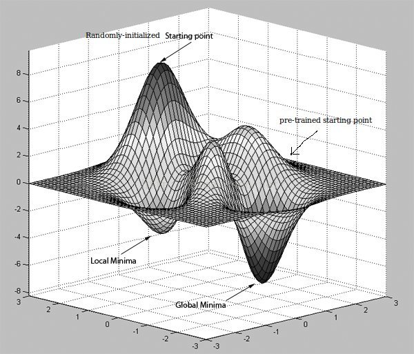
What network pre-training do is to bring the initialization points to a better point that has more possibility to reach a better minimum point. 

Here is a good picture to illustrate this:

(Reference: http://stackoverflow.com/questions/34514687/how-does-pre-training-improve-classification-in-neural-networks)

  

There are two interesting images come from this website:

Now, I will introduce what autocoder do:

(Reference: http://www.cnblogs.com/rong86/p/3555290.html)

Different from normal supervised training during which training dataset has its own labels. The error computation of autocoder is:

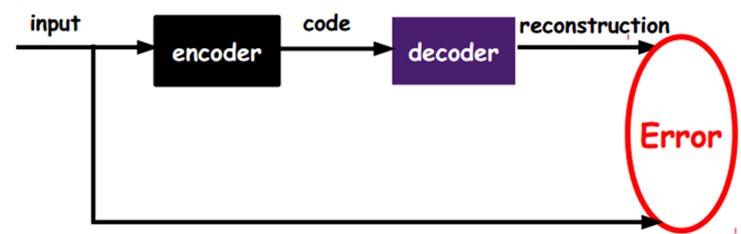
How we pre-train our network is to let a particular one layer become the encoder we design. And we manually introduce a decoder in it. If the encoder's output did not well present the input. Then we need to adjust the parameters of this layer. 

There are many autocoders have more complex architecture like sparse auto-encoder and de-noising auto-encoder.

2/ How to let the parameters matrix(θ) sparse 

At first, I would like to talk about why should we make the θ sparse. When we are talking about sparse, we are hoping that the matrix has more zeros in it. If a matrix has more zeros, the layer it belongs will be more anti-disturb because this layer will focus on the 'important' features of the input. 

Another perspective to understand this is that a sparser parameters' matrix will have a more smooth decision boundary since some items of polynomial are zero. This will be more likely to prevent over-fitting. 

------

Here is a good understanding from http://blog.csdn.net/zouxy09/article/details/24971995 and I quote (Chinese): 

监督机器学习问题无非就是“minimize your error while regularizing your parameters”，也就是在规则化参数的同时最小化误差。最小化误差是为了让我们的模型拟合我们的训练数据，而规则化参数是防止我们的模型过分拟合我们的训练数据。多么简约的哲学啊！因为参数太多，会导致我们的模型复杂度上升，容易过拟合，也就是我们的训练误差会很小。但训练误差小并不是我们的最终目标，我们的目标是希望模型的测试误差小，也就是能准确的预测新的样本。所以，我们需要保证模型“简单”的基础上最小化训练误差，这样得到的参数才具有好的泛化性能（也就是测试误差也小).

------

How to make the parameters' matrix sparse?

(1) Choose the right activation function:

(Reference: http://www.cnblogs.com/neopenx/p/4453161.html)

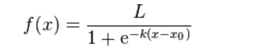
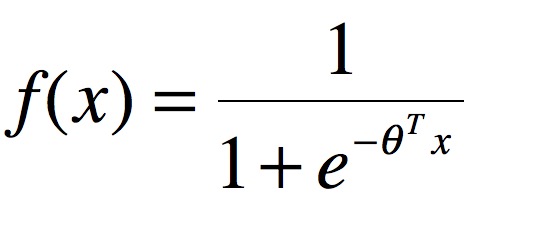
Sigmoid function: 

They are traditional function of sigmoid: Logistic-Sigmoid/ Tanh-Sigmoid. 

The expression are: 

Logistic-Sigmoid: 

Tanh-Sigmoid: 

---

From http://www.cnblogs.com/neopenx/p/4453161.html:

从数学上来看，非线性的Sigmoid函数对中央区的信号增益较大，对两侧区的信号增益小，在信号的特征空间映射上，有很好的效果。


从神经科学上来看，中央区酷似神经元的兴奋态，两侧区酷似神经元的抑制态，因而在神经网络学习方面，可以将重点特征推向中央区，将非重点特征推向两侧区。

---

Softplus and Rectifier Linear Unit(ReLU) 

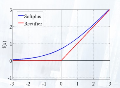
Softplus(x)=log(1+ex)

ReLU = max(0,x). 

Actually, in neural science research: 

---

From http://www.cnblogs.com/neopenx/p/4453161.html

在神经科学方面，除了新的激活频率函数之外，神经科学家还发现了神经元的稀疏激活性。

还是2001年，Attwell等人基于大脑能量消耗的观察学习上，推测神经元编码工作方式具有稀疏性和分布性。

2003年Lennie等人估测大脑同时被激活的神经元只有1~4%，进一步表明神经元工作的稀疏性。

从信号方面来看，即神经元同时只对输入信号的少部分选择性响应，大量信号被刻意的屏蔽了，这样可以提高学习的精度，更好更快地提取稀疏特征。

从这个角度来看，在经验规则的初始化W之后，传统的Sigmoid系函数同时近乎有一半的神经元被激活，这不符合神经科学的研究，而且会给深度网络训练带来巨大问题。

Softplus照顾到了新模型的前两点，却没有稀疏激活性。因而，校正函数 max(0,x) 成了近似符合该模型的最大赢家。

撇开稀疏激活不谈，校正激活函数 max(0,x) ，与Softplus函数在兴奋端的差异较大(线性和非线性)。

几十年的机器学习发展中，我们形成了这样一个概念：非线性激活函数要比线性激活函数更加先进。

尤其是在布满Sigmoid函数的BP神经网络，布满径向基函数的SVM神经网络中，往往有这样的幻觉，非线性函数对非线性网络贡献巨大。

该幻觉在SVM中更加严重。核函数的形式并非完全是SVM能够处理非线性数据的主力功臣（支持向量充当着隐层角色）。

那么在深度网络中，对非线性的依赖程度就可以缩一缩。另外，在上一部分提到，稀疏特征并不需要网络具有很强的处理线性不可分机制。

综合以上两点，在深度学习模型中，使用简单、速度快的线性激活函数可能更为合适。

一旦神经元与神经元之间改为线性激活，网络的非线性部分仅仅来自于神经元部分选择性激活。

Also max(0,x) can address the vanishing gradient problem of sigmoid: 

更倾向于使用线性神经激活函数的另外一个原因是，减轻梯度法训练深度网络时的Vanishing Gradient Problem。

看过BP推导的人都知道，误差从输出层反向传播算梯度时，在各层都要乘当前层的输入神经元值，激活函数的一阶导数。

即 Grad=Error⋅Sigmoid′(x)⋅x 。使用双端饱和(即值域被限制)Sigmoid系函数会有两个问题：

①Sigmoid'(x)∈(0,1)  导数缩放

②x∈(0,1)或x∈(-1,1)  饱和值缩放

这样，经过每一层时，Error都是成倍的衰减，一旦进行递推式的多层的反向传播，梯度就会不停的衰减，消失，使得网络学习变慢。

而校正激活函数的梯度是1，且只有一端饱和，梯度很好的在反向传播中流动，训练速度得到了很大的提高。

Softplus函数则稍微慢点，Softplus'(x)=Sigmoid(x)∈(0,1) ，但是也是单端饱和，因而速度仍然会比Sigmoid系函数快。

---

(2) Regulation

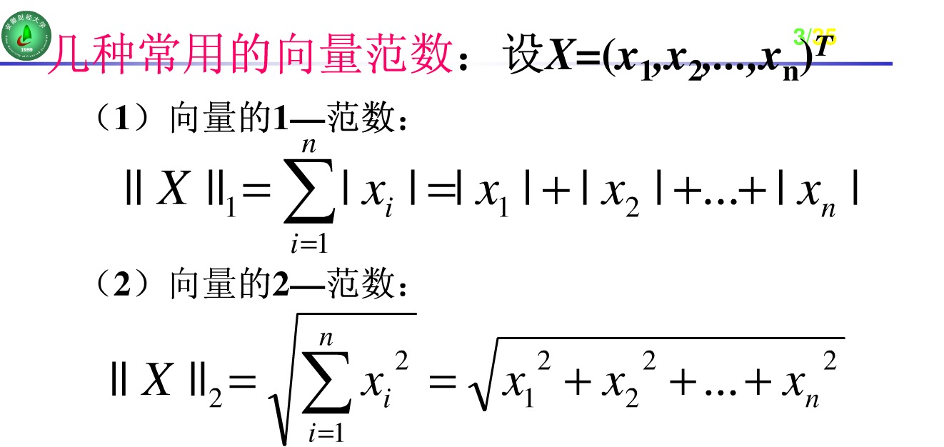
2.1 L0, L1 and L2 norm

First, let me introduce what is L0, L1 and L2 norm. 

L0 norm is number of zero in matrix w. L1 and L2 have a good picture to show: 

The update function of supervised learning is: 

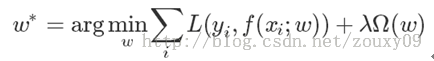
Normally, we will introduce L0, L1 and L2 norm to Ω(w). Particularly, L2 norm has another name call 'weight decay'. Being different from L0 and L1, L2 just regularize the parameters to small but not zero. 

A detailed explanation of those is: http://blog.csdn.net/zouxy09/article/details/24971995

(wait for continue)