


算法思想
粒子群算法(Particle Swarm Optimization)


优点:
1)原理比较简单,实现容易,参数少。
缺点:
1)易早熟收敛至局部最优、迭代后期收敛速度慢的。
算法拓展
针对标准PSO的缺点,通常有如下的改进:
- 实现参数的自适应变化。
- 引入一些其他机制。比如随机的因素,速度、位置的边界变化-后期压缩最大速度等。
- 结合其他智能优化算法:遗传算法、免疫算法、模拟退火算法等等,帮助粒子跳出局部最优,改善收敛速度。
matlab代码
二维下
%% 初始化种群
clear
%% Sphere
clear
f= @(x) x .* sin(x) .* cos(2 * x) - 2 * x .* sin(3 * x) +3 * x .* sin(4 * x); % 函数表达式    % 求这个函数的最大值


N = 20;                         % 初始种群个数
d = 1;                          % 可行解维数
ger = 100;                      % 最大迭代次数
limit = [0, 50];               % 设置位置参数限制
vlimit = [-10, 10];               % 设置速度限制
w = 0.8;                        % 惯性权重
c1 = 0.5;                       % 自我学习因子
c2 = 0.5;                       % 群体学习因子
figure(1);ezplot(f,[0,0.01,limit(2)]);   %曲线

x = limit(1) + (  limit( 2 ) -  limit( 1)  ) .* rand(N, d);%初始种群的位置

v = rand(N, d);                  % 初始种群的速度
xm = x;                          % 每个个体的历史最佳位置
ym = zeros(1, d);                % 种群的历史最佳位置
fxm = ones(N, 1)*inf;               % 每个个体的历史最佳适应度
fym = inf;                       % 种群历史最佳适应度
hold on
plot(xm, f(xm), 'ro');title('初始状态图');
figure(2)
%% 群体更新
iter = 1;
% record = zeros(ger, 1);          % 记录器
while iter <= ger
     fx = f(x) ; % 个体当前适应度
     for i = 1:N
        if fx(i)  <fxm(i)
            fxm(i) = fx(i);     % 更新个体历史最佳适应度
            xm(i,:) = x(i,:);   % 更新个体历史最佳位置(取值第i行的所有列)
        end
     end
    if  min(fxm)  < fym
        [fym, nmin] = min(fxm);   % 更新群体历史最佳适应度
        ym = xm(nmin, :);      % 更新群体历史最佳位置
    end
    v = v * w + c1 * rand * (xm - x) + c2 * rand * (repmat(ym, N, 1) - x);% 速度更新
    % 边界速度处理
    v(v > vlimit(2)) = vlimit(2);  %可以根据括号中的条件决定是否赋值
    v(v < vlimit(1)) = vlimit(1);
    x = x + v;% 位置更新
    % 边界位置处理
    x(x > limit(2)) = limit(2);
    x(x < limit(1)) = limit(1);
    record(iter) = fym;%最大值记录
    x0 = 0 : 0.01 : limit(2);  %1行3列的数组
    subplot(1,2,1)
    plot(x0, f(x0), 'b-', x, f(x), 'ro');title('状态位置变化')
    subplot(1,2,2);plot(record);title('最优适应度进化过程')
    pause(0.01)
    iter = iter+1;

end

x0 = 0 : 0.01 : limit(2);
figure(4);plot(x0, f(x0), 'b-', x, f(x), 'ro');title('最终状态位置')
disp(['最大值:',num2str(fym)]);
disp(['变量取值:',num2str(ym)]);


三维下
%% 初始化种群
clear
clc
f = @(x,y)   20 +  x.^2 + y.^2 - 10*cos(2*pi.*x)  - 10*cos(2*pi.*y) ;%[-5.12 ,5.12 ]


x0 = [-5.12:0.05:5.12];
y0 = x0 ;
[X,Y] = meshgrid(x0,y0);
Z =f(X,Y)  ;
figure(1); mesh(X,Y,Z);
colormap(parula(5));

N = 50;                         % 初始种群个数
d = 2;                          % 可行解维数
ger = 100;                      % 最大迭代次数
limit = [-5.12,5.12];               % 设置位置参数限制
vlimit = [-.5, .5];               % 设置速度限制
w = 0.8;                        % 惯性权重
c1 = 0.5;                       % 自我学习因子
c2 = 0.5;                       % 群体学习因子


x = limit(1) + (  limit( 2 ) -  limit( 1)  ) .* rand(N, d);%初始种群的位置

v = rand(N, d);                  % 初始种群的速度
xm = x;                          % 每个个体的历史最佳位置
ym = zeros(1, d);                % 种群的历史最佳位置
fxm = ones(N, 1)*inf;               % 每个个体的历史最佳适应度
fym = inf;                       % 种群历史最佳适应度
% record = zeros(ger,1);
hold on
% [X,Y] = meshgrid(x(:,1),x(:,2));
% Z = f( X,Y ) ;
scatter3( x(:,1),x(:,2) ,f( x(:,1),x(:,2) ),'r*' );
figure(2)
record=[];

%% 群体更新
iter = 1;
% record = zeros(ger, 1);          % 记录器
while iter <= ger
     fx = f( x(:,1),x(:,2) ) ;% 个体当前适应度
     for i = 1:N
        if  fx(i)  <fxm(i)
            fxm(i) = fx(i);     % 更新个体历史最佳适应度
            xm(i,:) = x(i,:);   % 更新个体历史最佳位置(取值)
        end
     end
    if   min(fxm)<  fym
        [fym, nmin] = min(fxm);   % 更新群体历史最佳适应度
        ym = xm(nmin, :);      % 更新群体历史最佳位置
    end
    v = v * w + c1 * rand * (xm - x) + c2 * rand * (repmat(ym, N, 1) - x);% 速度更新
    % 边界速度处理
    v(v > vlimit(2)) = vlimit(2);
    v(v < vlimit(1)) = vlimit(1);
    x = x + v;% 位置更新
    % 边界位置处理
    x(x > limit(2)) = limit(2);
    x(x < limit(1)) = limit(1);
    record(iter) = fym;%最大值记录
    subplot(1,2,1)
    mesh(X,Y,Z)
    hold on
    scatter3( x(:,1),x(:,2) ,f( x(:,1),x(:,2) ) ,'r*');title(['状态位置变化','-迭代次数:',num2str(iter)])
    subplot(1,2,2);plot(record);title('最优适应度进化过程')
    pause(0.01)
    iter = iter+1;

end

figure(4);mesh(X,Y,Z); hold on
scatter3( x(:,1),x(:,2) ,f( x(:,1),x(:,2) ) ,'r*');title('最终状态位置')
disp(['最优值:',num2str(fym)]);
disp(['变量取值:',num2str(ym)]);


python代码
import numpy as np
import matplotlib.pyplot as plt
# 粒子(鸟)
class particle:
def __init__(self):
self.pos = 0 # 粒子当前位置
self.speed = 0
self.pbest = 0 # 粒子历史最好位置
class PSO:
def __init__(self):
self.w = 0.5 # 惯性因子
self.c1 = 1 # 自我认知学习因子
self.c2 = 1 # 社会认知学习因子
self.gbest = 0 # 种群当前最好位置
self.N = 20 # 种群中粒子数量
self.POP = [] # 种群
self.iter_N = 100 # 迭代次数
# 适应度值计算函数
def fitness(self, x):
return x + 16 * np.sin(5 * x) + 10 * np.cos(4 * x)
# 找到全局最优解
def g_best(self, pop):
for bird in pop:
if bird.fitness > self.fitness(self.gbest):
self.gbest = bird.pos
# 初始化种群
def initPopulation(self, pop, N):
for i in range(N):
bird = particle()#初始化鸟
bird.pos = np.random.uniform(-10, 10)#均匀分布
bird.fitness = self.fitness(bird.pos)
bird.pbest = bird.fitness
pop.append(bird)
# 找到种群中的最优位置
self.g_best(pop)
# 更新速度和位置
def update(self, pop):
for bird in pop:
# 速度更新
speed = self.w * bird.speed + self.c1 * np.random.random() * (
bird.pbest - bird.pos) + self.c2 * np.random.random() * (
self.gbest - bird.pos)
# 位置更新
pos = bird.pos + speed
if -10 < pos < 10: # 必须在搜索空间内
bird.pos = pos
bird.speed = speed
# 更新适应度
bird.fitness = self.fitness(bird.pos)
# 是否需要更新本粒子历史最好位置
if bird.fitness > self.fitness(bird.pbest):
bird.pbest = bird.pos
# 最终执行
def implement(self):
# 初始化种群
self.initPopulation(self.POP, self.N)
# 迭代
for i in range(self.iter_N):
# 更新速度和位置
self.update(self.POP)
# 更新种群中最好位置
self.g_best(self.POP)
pso = PSO()
pso.implement()
best_x=0
best_y=0
for ind in pso.POP:
#print("x=", ind.pos, "f(x)=", ind.fitness)
if ind.fitness>best_y:
best_y=ind.fitness
best_x=ind.pos
print(best_y)
print(best_x)
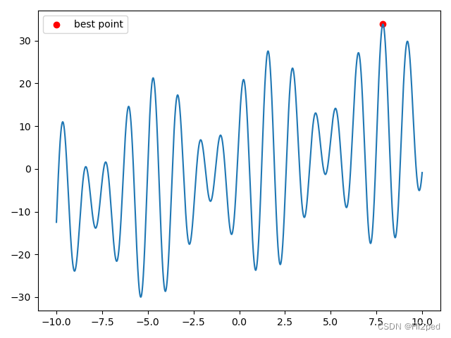
x = np.linspace(-10, 10, 100000)
def fun(x):
return x + 16 * np.sin(5 * x) + 10 * np.cos(4 * x)
y=fun(x)
plt.plot(x, y)
plt.scatter(best_x,best_y,c='r',label='best point')
plt.legend()
plt.show()
注:
算法思想和matlab代码来自于
【通俗易懂讲算法-最优化之粒子群优化(PSO)】
python代码来自于
粒子群PSO优化算法学习笔记 及其python实现(附讲解如何使用python语言sko.PSO工具包)


 1505
1505


 被折叠的 条评论
为什么被折叠?
被折叠的 条评论
为什么被折叠?
 到【灌水乐园】发言


