


 本项目基于Python分析2013-2018年全国城市空气质量,揭示了全国及广东省、深圳市的污染状况、主要污染物和季节性变化。结果显示,北部内陆和西北部空气质量较差,而沿海和高原地区较好。全国最差的10个省份主要污染物是pm10、so2、no2,冬季污染最严重。广东省主要污染物为pm2.5、pm10,深圳市空气质量在全国排名38位。
基于Python的2013-2018全国城市空气质量分析
项目摘要
本项目使用pandas/numpy工具包对557424条空气质量数据进行导入及清洗,并使用matplotlib/seaborn/pyecharts工具包可视化分析全国主要省市的空气质量情况,对空气质量最差及最好的省市进行排名,利用相关性分析省市的主要污染物,从不同层面给出污染物指标控制方案。
主要结论如下:
- 中国北部内陆地区以及西北部地区空气质量较差,沿海地区及高原地区空气质量较好;
- 全国空气质量最差的10个省份(排名分先后,差-好):河北省、北京、河南省、天津、新疆、山东、山西、陕西、江苏、湖北;
- 全国空气质量最好的10个省份(排名分先后,好-差):海南、云南、福建、贵州、西藏、广东、广西、黑龙江、江西、青海;
- 全国空气质量最差的10个城市/地区(排名分先后,差-好):和田地区、喀什地区、保定、邢台、阿克苏地区、石家庄、克牧勒苏州、衡水、邯郸;
- 全国空气质量最好的10个城市/地区(排名分先后,好-差):三亚、迪庆州、海口、丽江、黔西南州、怒江州、阿坝州、楚雄州、大理州、普洱;
- 空气质量最差省份的主要污染物是pm10、so2、no2。so2与no2两者正相关;
- 空气质量最差城市的主要污染物是pm2.5、pm10、so2、no2。so2与no2之间、pm2.5与pm10、so2、no2之间有较强的正相关关系;
- 全国空气质量冬季时最差,平均AQI为101.6(轻度污染),夏季时最好,平均AQI为71.9(良好);
- 2015年后全国空气质量有很大改善,特别是2016年~2018年,平均AQI约为80,较2013年下降40%;
- 广东省最主要的污染物是pm2.5、pm10,其次是so2、no2、co;
- 广东省21个城市中,佛山、东莞、广州空气质量最差,AQI分别为73、73.5、74.2,空气质量均为良;
- 广东省冬季AQI较高,空气质量较差,夏季AQI较低,空气质量较好; 广东省空气质量全国排名第6;
- 深圳市主要的污染物是pm2.5、pm10、so2、co; 深圳市空气质量在全国城市空气质量排名38位。
1.项目背景
本项目以2013-2018年的全国城市空气质量历史数据作为依据,探究全国空气质量与各污染物之间的联系。
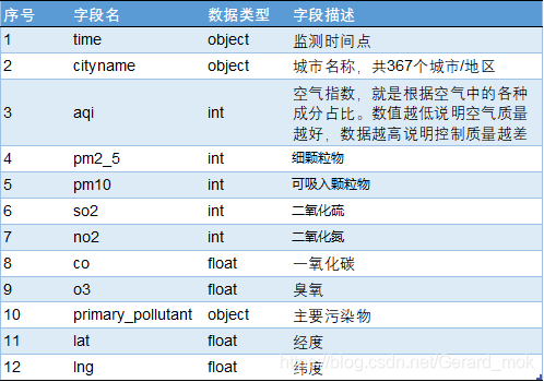
2.数据集介绍
数据集地址:https://tianchi.aliyun.com/dataset/dataDetail?dataId=2881
数据来自阿里天池,作者通过PythonSpider从真气网获取数据。以下为各字段描述:
3.项目分析
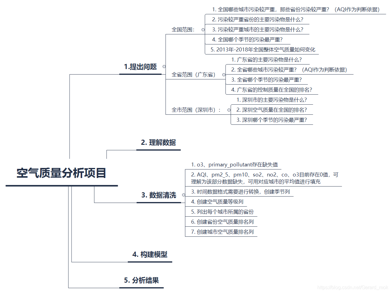
3.1 提出问题
全国范围:
- 全国哪些城市污染较严重,那些省份污染较严重?(AQI作为判断依据)
- 污染较严重省份的主要污染物是什么?
- 污染较严重城市的主要污染物是什么?
- 全国哪个季节的污染最严重?
- 2013年-2018年全国整体空气质量如何变化
全省范围(广东省):
- 广东省的主要污染物是什么?
- 全省哪些城市污染较严重?(AQI作为判断依据)
- 全省哪个季节的污染最严重?
- 广东省的控制质量在全国的排名?
全市范围(深圳市):
- 深圳市的主要污染物是什么?
- 深圳空气质量在全国的排名?
- 深圳哪个季节的污染最严重?
3.2 理解数据
import pandas as pd
import numpy as np
import seaborn as sns
import matplotlib.pyplot as plt
%matplotlib inline
df = pd.read_csv('aqi_data_u.csv')
df.head() # 查看表格
| time | cityname | aqi | pm2_5 | pm10 | so2 | no2 | co | o3 | primary_pollutant | |
|---|---|---|---|---|---|---|---|---|---|---|
| 0 | 2014-12-31 | 阿坝州 | 53 | 33 | 55 | 3 | 23 | 1.0 | 35.0 | PM10 |
| 1 | 2015-01-31 | 阿坝州 | 31 | 18 | 29 | 7 | 10 | 0.5 | 45.0 | NaN |
| 2 | 2015-01-30 | 阿坝州 | 34 | 19 | 30 | 7 | 13 | 0.6 | 48.0 | NaN |
| 3 | 2015-01-29 | 阿坝州 | 31 | 18 | 31 | 7 | 15 | 0.5 | 32.0 | NaN |
| 4 | 2015-01-28 | 阿坝州 | 29 | 18 | 29 | 7 | 14 | 0.6 | 27.0 | NaN |
df1 = pd.read_csv('city.csv')
df1.head() # 查看表格。此表为坐标表格,本项目后续改进时增加地图显示城市空气质量
| city | lat | lng | |
|---|---|---|---|
| 0 | 阿坝州 | 31.905763 | 102.228565 |
| 1 | 安康 | 32.704370 | 109.038045 |
| 2 | 阿克苏地区 | 41.171731 | 80.269846 |
| 3 | 阿里地区 | 30.404557 | 81.107669 |
| 4 | 阿拉善盟 | 38.843075 | 105.695683 |
df1.rename(columns={
   'city': 'cityname'}, inplace=True) # 重命名city列,以对应df表的列名
df1.head()
| cityname | lat | lng | |
|---|---|---|---|
| 0 | 阿坝州 | 31.905763 | 102.228565 |
| 1 | 安康 | 32.704370 | 109.038045 |
| 2 | 阿克苏地区 | 41.171731 | 80.269846 |
| 3 | 阿里地区 | 30.404557 | 81.107669 |
| 4 | 阿拉善盟 | 38.843075 | 105.695683 |
df = pd.merge(df, df1, on='cityname', how='inner') # 两个表格合并
df.head()
| time | cityname | aqi | pm2_5 | pm10 | so2 | no2 | co | o3 | primary_pollutant | lat | lng | |
|---|---|---|---|---|---|---|---|---|---|---|---|---|
| 0 | 2014-12-31 | 阿坝州 | 53 | 33 | 55 | 3 | 23 | 1.0 | 35.0 | PM10 | 31.905763 | 102.228565 |
| 1 | 2015-01-31 | 阿坝州 | 31 | 18 | 29 | 7 | 10 | 0.5 | 45.0 | NaN | 31.905763 | 102.228565 |
| 2 | 2015-01-30 | 阿坝州 | 34 | 19 | 30 | 7 | 13 | 0.6 | 48.0 | NaN | 31.905763 | 102.228565 |
| 3 | 2015-01-29 | 阿坝州 | 31 | 18 | 31 | 7 | 15 | 0.5 | 32.0 | NaN | 31.905763 | 102.228565 |
| 4 | 2015-01-28 | 阿坝州 | 29 | 18 | 29 | 7 | 14 | 0.6 | 27.0 | NaN | 31.905763 | 102.228565 |
df.shape # 查看数据数量
(557424, 12)
共557424行,12列数据。
df.describe()
| aqi | pm2_5 | pm10 | so2 | no2 | co | o3 | lat | lng | |
|---|---|---|---|---|---|---|---|---|---|
| count | 557424.000000 | 557424.000000 | 557424.000000 | 557424.000000 | 557424.000000 | 557424.000000 | 211516.000000 | 557424.000000 | 557424.000000 |
| mean | 82.604734 | 48.958870 | 84.865831 | 22.943201 | 31.041986 | 1.309690 | 77.638103 | 33.320514 | 112.931476 |
| std | 49.948024 | 235.684284 | 74.218273 | 25.620462 | 18.087321 | 49.111775 | 62.773975 | 6.583132 | 9.278219 |
| min | 0.000000 | 0.000000 | 0.000000 | 0.000000 | 0.000000 | 0.000000 | 0.000000 | 18.257776 | 75.992973 |
| 25% | 52.000000 | 23.000000 | 44.000000 | 9.000000 | 18.000000 | 0.700000 | 42.000000 | 28.668283 | 108.069948 |
| 50% | 71.000000 | 37.000000 | 68.000000 | 15.000000 | 27.000000 | 0.900000 | 69.000000 | 32.929499 | 114.351807 |
| 75% | 99.000000 | 60.000000 | 106.000000 | 27.000000 | 40.000000 | 1.200000 | 102.000000 | 37.661160 | 119.455835 |
| max | 1210.000000 | 65535.000000 | 12060.000000 | 1495.000000 | 574.000000 | 9999.900000 | 11281.000000 | 51.991789 | 131.171402 |
df.info()
<class 'pandas.core.frame.DataFrame'>
Int64Index: 557424 entries, 0 to 557423
Data columns (total 12 columns):
time                 557424 non-null object
cityname             557424 non-null object
aqi                  557424 non-null int64
pm2_5                557424 non-null int64
pm10                 557424 non-null int64
so2                  557424 non-null int64
no2                  557424 non-null int64
co                   557424 non-null float64
o3                   211516 non-null float64
primary_pollutant    528587 non-null object
lat                  557424 non-null float64
lng                  557424 non-null float64
dtypes: float64(4), int64(5), object(3)
memory usage: 55.3+ MB
print('数据中的城市数量为:', df.cityname.value_counts().count())
数据中的城市数量为: 367
3.3 数据清洗
根据以上简单查看数据,得出以下数据清洗思路:
1.o3、primary_pollutant存在缺失值。o3使用所在城市平均值填充,primary_pollutant统计数据较混乱且与项目问题无关,删除此列;
2.AQI、pm2_5、pm10、so2、no2、co、o3目前存在0值,可理解为该部分数据缺失,可用对应城市的平均值进行填充;
3.时间数据格式需要进行转换,创建季节列;
4.创建空气质量等级列;
5.列出每个城市所属的省份;
6.创建省份空气质量排名列(以AQI为基础);
7.创建城市空气质量排名列(以AQI为基础)。
# 1.o3、primary_pollutant存在缺失值。o3使用所在城市平均值填充,
# primary_pollutant统计数据较混乱且与项目问题无关,删除此列;
for city in df.cityname.value_counts().index:
    '''
    for循环计算每个城市污染物的平均值后替换NaN值
    '''
    df.loc[(df['cityname'] == city) & (df['o3'].isnull()), 'o3'] = df[df['cityname'] == city]['o3'].mean()

df['o3'].isnull().sum()
0
填充后缺失值为0
df.drop(['primary_pollutant'], axis=1, inplace=True)
df.head() #查看调整后的表格
| time | cityname | aqi | pm2_5 | pm10 | so2 | no2 | co | o3 | lat | lng | |
|---|---|---|---|---|---|---|---|---|---|---|---|
| 0 | 2014-12-31 | 阿坝州 | 53 | 33 | 55 | 3 | 23 | 1.0 | 35.0 | 31.905763 | 102.228565 |
| 1 | 2015-01-31 | 阿坝州 | 31 | 18 | 29 | 7 | 10 | 0.5 | 45.0 | 31.905763 | 102.228565 |
| 2 | 2015-01-30 | 阿坝州 | 34 | 19 | 30 | 7 | 13 | 0.6 | 48.0 | 31.905763 | 102.228565 |
| 3 | 2015-01-29 | 阿坝州 | 31 | 18 | 31 | 7 | 15 | 0.5 | 32.0 | 31.905763 | 102.228565 |
| 4 | 2015-01-28 | 阿坝州 | 29 | 18 | 29 | 7 | 14 | 0.6 | 27.0 | 31.905763 | 102.228565 |
df.isnull().any() # 确认表格中是否还有缺失值
time        False
cityname    False
aqi         False
pm2_5       False
pm10        False
so2         False
no2         False
co          False
o3          False
lat         False
lng         False
dtype: bool
# 2.AQI、pm2_5、pm10、so2、no2、co、o3目前存在0值,可理解为该部分数据缺失,可用对应城市的平均值进行填充;
df[['aqi', 'pm2_5', 'pm10', 'so2', 'no2', 'co', 'o3']] = df[['aqi', 'pm2_5', 'pm10', 'so2',
                                                             'no2', 'co', 'o3']].replace(0, np.NaN)
df.isnull().sum() # 将0值替换后缺失值的数量
time           0
cityname       0
aqi         4199
pm2_5       6817
pm10        4817
so2         1631
no2         1621
co          3493
o3          2342
lat            0
lng            0
dtype: int64
cities = df.cityname.value_counts().index
for city in cities:
    '''
    for循环计算每个城市污染物的平均值后替换NaN值
    '''
    for pollutant in ['aqi', 'pm2_5', 'pm10', 'so2', 'no2', 'co', 'o3']:
        df.loc[(df['cityname'] == city) & (df[pollutant].isnull()), pollutant] = df[df['cityname'] == city][pollutant].mean()
df.isnull().sum() # 再次检查缺失值
time        0
cityname    0
aqi         0
pm2_5       0
pm10        0
so2         0
no2         0
co          0
o3          0
lat         0
lng         0
dtype: int64
# 3.时间数据格式需要进行转换,创建季节列;
df['time'] = pd.to_datetime(df['time'])
df.info() #查看time列的数据类型
<class 'pandas.core.frame.DataFrame'>
Int64Index: 557424 entries, 0 to 557423
Data columns (total 11 columns):
time        557424 non-null datetime64[ns]
cityname    557424 non-null object
aqi         557424 non-null float64
pm2_5       557424 non-null float64
pm10        557424 non-null float64
so2         557424 non-null float64
no2         557424 non-null float64
co          557424 non-null float64
o3          557424 non-null float64
lat         557424 non-null float64
lng         557424 non-null float64
dtypes: datetime64[ns](1), float64(9), object(1)
memory usage: 51.0+ MB
# 根据月份创建季节列
seasons = {
   12: 'Winter',
           1: 'Winter',
           2: 'Winter',
           3: 'Spring',
           4: 'Spring',
           5: 'Spring',
           6: 'Summer',
           7: 'Summer',
           8: 'Summer',
           9: 'Autumn',
           10: 'Autumn',
           11: 'Autumn'
}
df['season'] = df['time'].apply(lambda x : seasons [x.month])
df.head()
| time | cityname | aqi | pm2_5 | pm10 | so2 | no2 | co | o3 | lat | lng | season | |
|---|---|---|---|---|---|---|---|---|---|---|---|---|
| 0 | 2014-12-31 | 阿坝州 | 53.0 | 33.0 | 55.0 | 3.0 | 23.0 | 1.0 | 35.0 | 31.905763 | 102.228565 | Winter |
| 1 | 2015-01-31 | 阿坝州 | 31.0 | 18.0 | 29.0 | 7.0 | 10.0 | 0.5 | 45.0 | 31.905763 | 102.228565 | Winter |
| 2 | 2015-01-30 | 阿坝州 | 34.0 | 19.0 | 30.0 | 7.0 | 13.0 | 0.6 | 48.0 | 31.905763 | 102.228565 | Winter |
| 3 | 2015-01-29 | 阿坝州 | 31.0 | 18.0 | 31.0 | 7.0 | 15.0 | 0.5 | 32.0 | 31.905763 | 102.228565 | Winter |
| 4 | 2015-01-28 | 阿坝州 | 29.0 | 18.0 | 29.0 | 7.0 | 14.0 | 0.6 | 27.0 | 31.905763 | 102.228565 | Winter |
# 4.创建空气质量等级列
bin_edges = [0, 50, 100, 150, 200, 300, 1210] # 根据AQI的划分等级设置标签
bin_names = ['优级', '良好', '轻度污染', '中度污染', '重度污染', '重污染']
df['空气质量'] = pd.cut(df['aqi'], bin_edges, labels=bin_names)
df.head()
| time | cityname | aqi | pm2_5 | pm10 | so2 | no2 | co | o3 | lat | lng | season | 空气质量 | |
|---|---|---|---|---|---|---|---|---|---|---|---|---|---|
| 0 | 2014-12-31 | 阿坝州 | 53.0 | 33.0 | 55.0 | 3.0 | 23.0 | 1.0 | 35.0 | 31.905763 | 102.228565 | Winter | 良好 |
| 1 | 2015-01-31 | 阿坝州 | 31.0 | 18.0 | 29.0 | 7.0 | 10.0 | 0.5 | 45.0 | 31.905763 | 102.228565 | Winter | 优级 |
| 2 | 2015-01-30 | 阿坝州 | 34.0 | 19.0 | 30.0 | 7.0 | 13.0 | 0.6 | 48.0 | 31.905763 | 102.228565 | Winter | 优级 |
| 3 | 2015-01-29 | 阿坝州 | 31.0 | 18.0 | 31.0 | 7.0 | 15.0 | 0.5 | 32.0 | 31.905763 | 102.228565 | Winter | 优级 |
| 4 | 2015-01-28 | 阿坝州 | 29.0 | 18.0 | 29.0 | 7.0 | 14.0 | 0.6 | 27.0 | 31.905763 | 102.228565 | Winter | 优级 |
# 5.列出每个城市所属的省份;

city_province={
   '即墨': '山东省', '阿坝州': '四川省', '安康': '陕西省', '阿克苏地区': '新疆维吾尔自治区',
               '阿里地区': '西藏区', '阿拉善盟': '内蒙古自治区', '安庆': '安徽省', '安顺': '贵州省', '鞍山': '辽宁省',
               '克孜勒苏州': '新疆维吾尔自治区', '安阳': '河南省', '蚌埠': '安徽省', '白城': '吉林省',
               '北海': '广西壮族自治区', '宝鸡': '陕西省', '毕节': '贵州省', '白山': '吉林省', '百色': '广西壮族自治区',
               '保山': '云南省', '包头': '内蒙古自治区', '本溪': '辽宁省', '巴彦淖尔': '内蒙古自治区',
               '白银': '甘肃省', '巴中': '四川省', '滨州': '山东省', '亳州': '安徽省', '昌都': '西藏区',
               '常德': '湖南省', '赤峰': '内蒙古自治区', '昌吉州': '新疆维吾尔自治区', '五家渠'<
最低0.47元/天 解锁文章


 482
482

 被折叠的 条评论
为什么被折叠?
被折叠的 条评论
为什么被折叠?
 到【灌水乐园】发言


