吴恩达作业（6）CNN神经网络(keras实现)-识别笑脸

参考博客
题目：
输入人脸图片，判断这个人开不开心。如：

开心输出$1$，不开心输出$0$
一个二分类问题

数据集：

1. test_happy.h5：
   训练集，维度为：（600，64，64，3），即600张64*64的彩色图片
2. train_happy.h5：
   测试集，维度为：（150，64，64，3），即150张64*64的彩色图片

参考博客

环境:
$tf$.__$version$__ = ‘$\mathrm{2.5.0}$’

目的：
搭建卷积层:
$CONV2D\stackrel{BatchNorm}{⟶}RELU⟶MAXPOOL⟶FLATTEN⟶FULLYCONNECTED⟶SIGMOID$

加载和处理数据

#加载和处理数据
def load_dataset():
    train_dataset = h5py.File('train_happy.h5', "r")
    train_set_x_orig = np.array(train_dataset["train_set_x"][:]) # your train set features
    train_set_y_orig = np.array(train_dataset["train_set_y"][:]) # your train set labels
    test_dataset = h5py.File('test_happy.h5', "r")
    test_set_x_orig = np.array(test_dataset["test_set_x"][:]) # your test set features
    test_set_y_orig = np.array(test_dataset["test_set_y"][:]) # your test set labels
    classes = np.array(test_dataset["list_classes"][:]) # the list of classes
    train_set_y_orig = train_set_y_orig.reshape((1, train_set_y_orig.shape[0]))
    test_set_y_orig = test_set_y_orig.reshape((1, test_set_y_orig.shape[0]))
    return train_set_x_orig, train_set_y_orig, test_set_x_orig, test_set_y_orig, classes

train_set_x_orig, train_set_y_orig, test_set_x_orig, test_set_y_orig, classes = load_dataset()
# Normalize image vectors
X_train = train_set_x_orig/255.
X_test = test_set_x_orig/255.

# Reshape
Y_train = train_set_y_orig.T
Y_test = test_set_y_orig.T
print('训练集样本维度：',train_set_x_orig.shape)
print('测试集样本维度：',test_set_x_orig.shape)

创建模型

from keras import Input,Model
from keras.layers import ZeroPadding2D,BatchNormalization,Conv2D,Activation,MaxPool2D,Flatten,Dense
def HappyModel(input_shape):
    #Input会自动创建一个palceholer,维度为input_shape
    X_input = Input(input_shape)
    
    #使用0进行padding
    X = ZeroPadding2D((3,3))(X_input)
    
    #卷积
    X = Conv2D(filters = 32,kernel_size = (7,7),strides=(1,1))(X)
    #Btach Norm
    X = BatchNormalization(axis=3,name='bn0')(X)
    #激活函数层
    X = Activation("relu")(X)
    
    #最大池化层
    X = MaxPool2D(pool_size=(2, 2),name="max_pool")(X)
    
    X = Flatten()(X)
    
    X = Dense(1, activation='sigmoid', name='fc')(X)
    
    model = Model(inputs=X_input, outputs=X, name='HappyModel')
    
    return model

函数讲解

一、输入层

tf.keras.Input(
    shape=None, batch_size=None, name=None, dtype=None, sparse=False, tensor=None,
    ragged=False, **kwargs
)

• $shape：integer$元组，(维度,样本数)
• $batc{h}_{s}ize：integer$ 一次输入的样本数量
• $name：string$ 在模型中要唯一不重复

二、$padding$函数，给图片最外层加$0$

tf.keras.layers.ZeroPadding2D(
    padding=(1, 1), data_format=None, **kwargs
)

• $padding$：
  $int\to$高度和宽度都以一个值进行填充
  (int,int) $\to$高度以第一个值进行填充，宽度以第二个值进行填充
  $((int,int),(int,int))\to ((top\_pad,bottom\_pad),(left\_pad,right\_pad))$

三、卷积层

tf.keras.layers.Conv2D(
    filters, kernel_size, strides=(1, 1), padding='valid', data_format=None,
    dilation_rate=(1, 1), activation=None, use_bias=True,
    kernel_initializer='glorot_uniform', bias_initializer='zeros',
    kernel_regularizer=None, bias_regularizer=None, activity_regularizer=None,
    kernel_constraint=None, bias_constraint=None, **kwargs
)

• $filters:Integer$ 过滤器数量
• $kernel\_size:Anintegerortuplelistorof2integers,(height,width)/[height,width]$
• $strides:Anintegerortupleorlistof2integers$ , 指定卷积沿高度和宽度的步长。
• $padding:"valid"or"same"$

四、Batch Norm

tf.keras.layers.BatchNormalization(
    axis=-1, momentum=0.99, epsilon=0.001, center=True, scale=True,
    beta_initializer='zeros', gamma_initializer='ones',
    moving_mean_initializer='zeros', moving_variance_initializer='ones',
    beta_regularizer=None, gamma_regularizer=None, beta_constraint=None,
    gamma_constraint=None, renorm=False, renorm_clipping=None, renorm_momentum=0.99,
    fused=None, trainable=True, virtual_batch_size=None, adjustment=None, name=None,
    **kwargs
)

• $axis：Integer,theaxisthatshouldbenormalized$ [批量，高度，宽度，通道]
• $momentum$ ：滑动平均的中的$betau=beta\ast u\_old+(1-beta)\ast u\_new$
• $epsilon：Smallfloataddedtovariancetoavoiddividingbyzero$.
• $center$：是否忽略$\beta$

五、激活函数

tf.keras.layers.Activation(
    activation, **kwargs
)

• $activation:tf.nn.relu或者"relu"$

六、最大池化

tf.keras.layers.MaxPool2D(
    pool_size=(2, 2), strides=None, padding='valid', data_format=None, **kwargs
)

• $pool\_size：integerortupleof2integers$
• $strides：Integer,tupleof2integersorNone$.
• $padding："valid"or"same"$

七、全连接层

tf.keras.layers.Dense(
    units, activation=None, use_bias=True, kernel_initializer='glorot_uniform',
    bias_initializer='zeros', kernel_regularizer=None, bias_regularizer=None,
    activity_regularizer=None, kernel_constraint=None, bias_constraint=None,
    **kwargs
)

• $units$:正整数 输出的维度
• $activation$：激活函数
• $use\_bias$：是否使用偏置向量

八、Model的参数

compile(
    optimizer='rmsprop', loss=None, metrics=None, loss_weights=None,
    weighted_metrics=None, run_eagerly=None, steps_per_execution=None, **kwargs
)

• $optimizer$:优化算法 $SGD:Gradientdescent(withmomentum)optimizer、RMSprop(rootmeansquareprop)、Adam$
• $loss$：$BinaryCrossentropy$(正负样本时使用) 、 $CategoricalCrossentropy$（预测值与真实值的交叉熵）、$MeanSquaredError$(平方根误差)

evaluate(
    x=None, y=None, batch_size=None, verbose=1, sample_weight=None, steps=None,
    callbacks=None, max_queue_size=10, workers=1, use_multiprocessing=False,
    return_dict=False, **kwargs
)

• $verbose：=0$时，不输出日志信息 $=1$时，带进度条的输出日志信息
• $batch\_size$:每次进行计算的样本数

模型运行

#创建一个模型实体
happy_model = HappyModel((64,64,3))
#编译模型
happy_model.compile(optimizer="adam",loss="binary_crossentropy", metrics=['accuracy'])

#训练模型
happy_model.fit(X_train, Y_train, epochs=40, batch_size=50)

#评估模型
preds = happy_model.evaluate(X_test, Y_test, batch_size=32)
print ("误差值 = " + str(preds[0]))
print ("准确度 = " + str(preds[1]))

运行结果

Epoch 1/40
12/12 [==============================] - 3s 185ms/step - loss: 1.6428 - accuracy: 0.5875
Epoch 2/40
12/12 [==============================] - 2s 172ms/step - loss: 0.4274 - accuracy: 0.8353
Epoch 3/40
12/12 [==============================] - 3s 212ms/step - loss: 0.2134 - accuracy: 0.9245
Epoch 4/40
12/12 [==============================] - 2s 173ms/step - loss: 0.1238 - accuracy: 0.9588
Epoch 5/40
12/12 [==============================] - 2s 148ms/step - loss: 0.1192 - accuracy: 0.9450
Epoch 6/40
12/12 [==============================] - 2s 139ms/step - loss: 0.0913 - accuracy: 0.9698
Epoch 7/40
12/12 [==============================] - 2s 165ms/step - loss: 0.1027 - accuracy: 0.9756
Epoch 8/40
12/12 [==============================] - 2s 203ms/step - loss: 0.0682 - accuracy: 0.9809
Epoch 9/40
12/12 [==============================] - 2s 157ms/step - loss: 0.0830 - accuracy: 0.9782
Epoch 10/40
12/12 [==============================] - 2s 142ms/step - loss: 0.0526 - accuracy: 0.9885
Epoch 11/40
12/12 [==============================] - 2s 137ms/step - loss: 0.0478 - accuracy: 0.9872
Epoch 12/40
12/12 [==============================] - 2s 145ms/step - loss: 0.0508 - accuracy: 0.9857
Epoch 13/40
12/12 [==============================] - 2s 132ms/step - loss: 0.0331 - accuracy: 0.9929
Epoch 14/40
12/12 [==============================] - 2s 141ms/step - loss: 0.0379 - accuracy: 0.9900
Epoch 15/40
12/12 [==============================] - 2s 138ms/step - loss: 0.0426 - accuracy: 0.9876
Epoch 16/40
12/12 [==============================] - 2s 143ms/step - loss: 0.0322 - accuracy: 0.9898
Epoch 17/40
12/12 [==============================] - 2s 143ms/step - loss: 0.0400 - accuracy: 0.9862
Epoch 18/40
12/12 [==============================] - 2s 161ms/step - loss: 0.0499 - accuracy: 0.9805
Epoch 19/40
12/12 [==============================] - 2s 152ms/step - loss: 0.0458 - accuracy: 0.9879
Epoch 20/40
12/12 [==============================] - 2s 142ms/step - loss: 0.0335 - accuracy: 0.9858
Epoch 21/40
12/12 [==============================] - 2s 147ms/step - loss: 0.0331 - accuracy: 0.9903
Epoch 22/40
12/12 [==============================] - 2s 159ms/step - loss: 0.0339 - accuracy: 0.9873
Epoch 23/40
12/12 [==============================] - 2s 158ms/step - loss: 0.0348 - accuracy: 0.9886
Epoch 24/40
12/12 [==============================] - 2s 145ms/step - loss: 0.0282 - accuracy: 0.9932
Epoch 25/40
12/12 [==============================] - 2s 150ms/step - loss: 0.0236 - accuracy: 0.9946
Epoch 26/40
12/12 [==============================] - 2s 174ms/step - loss: 0.0257 - accuracy: 0.9885
Epoch 27/40
12/12 [==============================] - 3s 261ms/step - loss: 0.0125 - accuracy: 0.9968
Epoch 28/40
12/12 [==============================] - 3s 210ms/step - loss: 0.0162 - accuracy: 0.9937
Epoch 29/40
12/12 [==============================] - 2s 198ms/step - loss: 0.0117 - accuracy: 0.9962
Epoch 30/40
12/12 [==============================] - 2s 175ms/step - loss: 0.0116 - accuracy: 0.9934
Epoch 31/40
12/12 [==============================] - 2s 176ms/step - loss: 0.0128 - accuracy: 0.9949
Epoch 32/40
12/12 [==============================] - 2s 189ms/step - loss: 0.0095 - accuracy: 0.9976
Epoch 33/40
12/12 [==============================] - 2s 161ms/step - loss: 0.0094 - accuracy: 0.9989
Epoch 34/40
12/12 [==============================] - 2s 192ms/step - loss: 0.0099 - accuracy: 0.9964
Epoch 35/40
12/12 [==============================] - 2s 177ms/step - loss: 0.0072 - accuracy: 1.0000
Epoch 36/40
12/12 [==============================] - 2s 197ms/step - loss: 0.0088 - accuracy: 0.9962
Epoch 37/40
12/12 [==============================] - 3s 229ms/step - loss: 0.0103 - accuracy: 0.9946
Epoch 38/40
12/12 [==============================] - 2s 191ms/step - loss: 0.0186 - accuracy: 0.9949
Epoch 39/40
12/12 [==============================] - 2s 186ms/step - loss: 0.0184 - accuracy: 0.9961
Epoch 40/40
12/12 [==============================] - 2s 195ms/step - loss: 0.0148 - accuracy: 0.9980
5/5 [==============================] - 0s 24ms/step - loss: 0.1235 - accuracy: 0.9533
误差值 = 0.12346960604190826
准确度 = 0.95333331823349

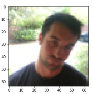
新图预测

from skimage import transform
boy = plt.imread('boy.jpeg')
boy = transform.resize(boy,(64,64))
plt.imshow(boy)
plt.show()

x = np.expand_dims(boy, axis=0)

print(happy_model.predict(x/255))

预测结果：

问题总结

• 多看官方tensorflow网站解决问题网址
• 测试数据与现实数据存在数据分布不匹配问题，模型并不能很好的预测网上的图片