


一、背景问题
在多径环境中,阵列接收的信号可能是相干的(例如,信号 \(s_2(t) = \alpha s_1(t)\)),导致信号协方差矩阵 \(\mathbf{R}_s\) 低秩(\(\text{rank}(\mathbf{R}_s) < D\),\(D\) 为信号源数)。这使得传统 MUSIC 算法无法正确分离信号和噪声子空间,谱峰丢失或模糊。
适用场景:均匀线阵(ULA),多径环境下的相干信号。
二、信号模型
信号模型在上一节详细介绍过,在此不多赘述。详见:MUSIC算法处理阵列信号的DOA估计-CSDN博客
三、Toeplitz 算法
3.1核心思想
- 从样本协方差矩阵 \(\hat{\mathbf{R}}_x\) 提取自相关序列 \(\hat{r}(k)\)。
- 用 \(\hat{r}(k)\) 构造 Hermitian Toeplitz 矩阵 \(\mathbf{R}_{\text{Toe}}\)。
- 用 \(\mathbf{R}_{\text{Toe}}\)近似非相干信号的协方差矩阵,恢复秩为 D 。
3.2算法步骤
1. 计算样本协方差矩阵:
$$
\hat{\mathbf{R}}_x = \frac{1}{N} \sum_{i=1}^N \mathbf{X}(i) \mathbf{X}^H(i)
$$
其中,\(N\) 为快拍数。
2. 提取自相关序列:
$$
\hat{r}(k) = \frac{1}{M-k} \sum_{m=0}^{M-k-1} \hat{\mathbf{R}}_x(m, m+k), \quad k = 0, 1, \dots, M-1
$$
确保 \(\mathbf{R}_{\text{Toe}}\) 矩阵的Hermitian 性质,从而实现特征分解:
$$
\hat{r}(-k) = \hat{r}^*(k)
$$
3. 构造 Toeplitz 矩阵:
矩阵元素定义为:
$$
\mathbf{R}_{\text{Toe}}(i,j) = \hat{r}(i-j)
$$
矩阵形式为:
$$
\mathbf{R}_{\text{Toe}} = \begin{bmatrix}
\hat{r}(0) & \hat{r}(1) & \cdots & \hat{r}(M-1) \\
\hat{r}^*(-1) & \hat{r}(0) & \cdots & \hat{r}(M-2) \\
\vdots & \vdots & \ddots & \vdots \\
\hat{r}^*(-(M-1)) & \hat{r}^*(-(M-2)) & \cdots & \hat{r}(0)
\end{bmatrix}
$$
4. 特征分解:
对 \(\mathbf{R}_{\text{Toe}}\) 进行特征分解:
$$
\mathbf{R}_{\text{Toe}} = \mathbf{U}_s \mathbf{\Lambda}_s \mathbf{U}_s^H + \mathbf{U}_n \mathbf{\Lambda}_n \mathbf{U}_n^H
$$
取噪声子空间 \(\mathbf{U}_n\)(后 \(M-D\) 列)。
5. 计算 MUSIC 谱:
$$
P_{\text{MUSIC}}(\theta) = \frac{1}{\mathbf{a}^H(\theta) \mathbf{U}_n \mathbf{U}_n^H \mathbf{a}(\theta)}
$$
峰值位置对应 AOA。
\(\mathbf{R}_{\text{Toe}}\) 近似非相干信号的协方差矩阵,恢复秩为 \(D\)。
注1:
\(\hat{r}(k)\) 的选取依据
为什么\(\hat{r}(k)\)满足:
$$
\hat{r}(k) = \frac{1}{M-k} \sum_{m=0}^{M-k-1} \hat{\mathbf{R}}_x(m, m+k), \quad k = 0, 1, \dots, M-1
$$
理论自相关序列
$$
r(k) = E[x_m(t) x_{m+k}^*(t)]
$$
- \(x_m(t)\):第 \(m\) 个阵元的接收信号。
- \(x_{m+k}(t)\):第 \(m+k\) 个阵元的接收信号。
- \(k\):空间滞后(阵元索引差)。
样本协方差矩阵的元素:
$$
\hat{\mathbf{R}}_x(m, n) = \frac{1}{N} \sum_{i=1}^N X_m(i) X_n^*(i)
$$
- \(X_m(i)\):第 \(i\) 个快拍中第 \(m\) 个阵元的信号。
物理意义:
$$
\hat{\mathbf{R}}_x(m, n) \approx E[x_m(t) x_n^*(t)]
$$
当 \(n = m+k\) 时:
$$
\hat{\mathbf{R}}_x(m, m+k) = \frac{1}{N} \sum_{i=1}^N X_m(i) X_{m+k}^*(i)
$$
这是阵元 \(m\) 和 \(m+k\) 的样本相关性,近似于 \(E[x_m(t) x_{m+k}^*(t)]\).
四、仿真代码
import numpy as np
import matplotlib.pyplot as plt
from scipy.signal import find_peaks

# 参数设置
M = 8
D = 2
d = 0.5
theta = [25, 50]
snr = 10
N = 100

# 方向向量函数(标准负相位)
def steering_vector(theta, M, d):
    theta_rad = np.deg2rad(theta)
    k = np.arange(M)
    return np.exp(-1j * 2 * np.pi * d * k * np.sin(theta_rad))

# MUSIC 谱函数
def music_spectrum(R, M, d, D):
    eigenvalues, U = np.linalg.eigh(R)
    idx = np.argsort(eigenvalues)[::-1]
    U = U[:, idx]
    U_n = U[:, D:]
    theta_range = np.linspace(-90, 90, 1000)
    P_music = []
    for th in theta_range:
        a = steering_vector(th, M, d)
        P_music.append(1 / np.abs(a.conj().T @ U_n @ U_n.conj().T @ a))
    return theta_range, np.array(P_music)

# 生成相干信号
A = np.array([steering_vector(t, M, d) for t in theta]).T
S = np.random.randn(D, N) + 1j * np.random.randn(D, N)
S[1, :] = 0.6 * S[0, :]
noise = (10**(-snr/20)) * (np.random.randn(M, N) + 1j * np.random.randn(M, N))
X = A @ S + noise

# 步骤 1:计算样本协方差矩阵
R_x = X @ X.conj().T / N

# 步骤 2:提取自相关序列
r = np.zeros(M, dtype=complex)
for k in range(M):
    r[k] = np.mean(np.diag(R_x,-k))

# 步骤 3:构造 Toeplitz 矩阵
R_toe = np.zeros((M, M), dtype=complex)
for i in range(M):
    for j in range(M):
        if i >= j:
            R_toe[i, j] = r[i - j]
        else:
            R_toe[i, j] = np.conj(r[j - i])
            # R_toe[i, j] = r[(abs(j - i))]

# 步骤 4 & 5:计算 MUSIC 谱
theta_range, P_music = music_spectrum(R_toe, M, d, D)

# 绘图
plt.plot(theta_range, 10 * np.log10(P_music))
plt.xlabel("Angle (degrees)")
plt.ylabel("MUSIC Spectrum (dB)")
plt.title("Toeplitz MUSIC for Coherent Signals")
for t in theta:
    plt.axvline(x=t, color='r', linestyle='--')
peaks, _ = find_peaks(10 * np.log10(P_music), height=0)
print("Detected peaks at:", theta_range[peaks])
plt.grid()
plt.show()
Toeplitz完成对相干信号的DOA估计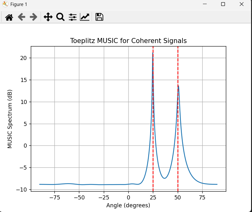 传统MUSIC算法则对相干信号的DOA混叠
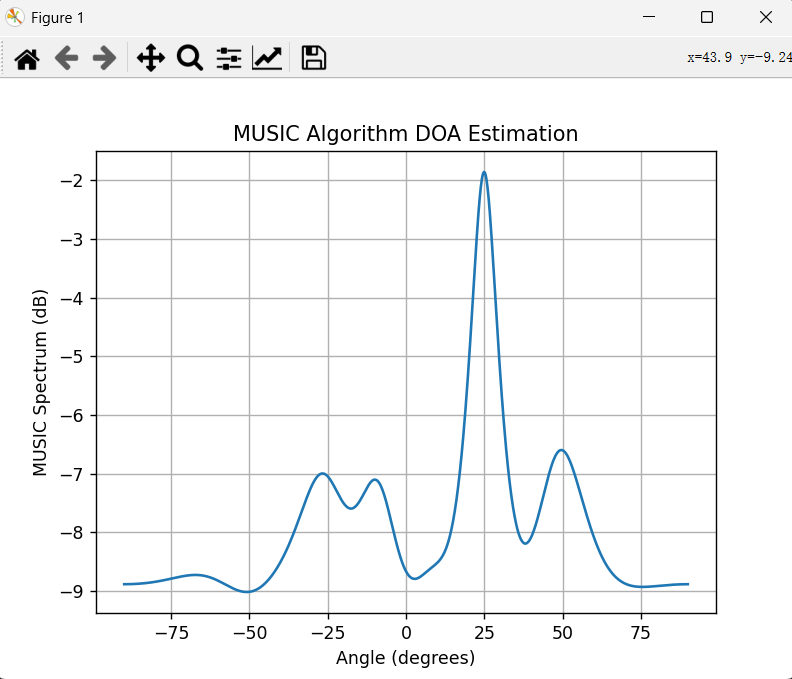


 496
496

 被折叠的 条评论
为什么被折叠?
被折叠的 条评论
为什么被折叠?
 到【灌水乐园】发言


