


Python与机器学习1:Numpy库(简笔记)
一、简介
1、AI之父:约翰·麦卡锡
2、相关概念:
	1、强AI(Strong AI)(Artificial General Intelligence)(Full AI)
		像人一样,可胜任智力性任务的智能机器。
	2、弱AI(Weak AI)(Narrow AI)(Applied AI)
		不具备智力 / 自我意识。
二、Numpy库
1、介绍

2、安装
	1、键盘 Win+R , 输入cmd
	2、命令行里输入 pip install numpy

3、运行
运行前记得 import numpy as np # 引入numpy的库 ,np为引入模块的别名。
dtype,d为data的缩写。
0、基础知识
# a 和 b 是什么类型 , 结果C打印输出是什么?
a = [1, 2, 3, 4, 5]
b = [1, 2, 3, 4, 5]
c = a + b
print(c)
print(type(a)) # 什么类型

# output:
[1, 2, 3, 4, 5, 1, 2, 3, 4, 5]
<class 'list'>
# 如何让c 输出结果是 [2, 4, 6, 8, 10]
a = [1,2,3,4,5]
b = [1,2,3,4,5]
c=[]
for i in range(len(a)):
	c1 = a[i] + b[i]
 	c.append(c1)  # 向列表末尾追加元素
print(c)

# output:
[2, 4, 6, 8, 10]
# 用numpy , 让c 输出结果是 [2, 4, 6, 8, 10]
import numpy as np
a = np.array([1, 2, 3, 4, 5])
b = np.array([1, 2, 3, 4, 5])
c = a + b
print(c)
1、创建 Numpy数组(基本函数)
(1) 从Python中的列表、元组等类型创建ndarray数组
1、np.array(任何可被解释为Numpy数组的逻辑结构,dtype=类型) ---> 任意维度和类型的数组对象
2、支持多维数组 + 各种运算函数
1.1.1 从列表类型创建
x = np.array([0,1,2,3])
print(x)
# [0 1 2 3]
1.1.2 从元组类型创建
x = np.array((4,5,6,7))
print(x)
# [4 5 6 7]
1.1.3 从列表和元组混合类型创建
x = np.array([ [1,2], [9,8], [0.1, 0.3] ])
print(x)
# [[1.  2. ]
#  [9.  8. ]
#  [0.1 0.3]]
1.1.4 np.array() 的功能
dtype : 数据类型(data type)
# 2、 np.array(任何可被解释为Numpy数组的逻辑结构,dtype=类型)--->任意维度和类型的数组对象
l = [[1,2,3],[4,5,6]] # 随便定义一个数组

# 强制把数组 l 转成一个【float类型 32位 】的数组 b
b = np.array(l, dtype=np.float32)
#   [ [1. 2. 3.]
#     [4. 5. 6.] ]
(2) 使用NumPy中函数创建ndarray数组,如: arange, ones, zeros等

1.2.1 np.arange() 【生成数组】
ndarray: n-dimension array 多维数组对象
# 1、 np.arange(start(0), end, step(1)) [括号里为默认值]

a1 = np.arange(1,10) # 左闭右开
print(a1)
# [1 2 3 4 5 6 7 8 9]

a2 = np.arange(1,10,2) # step为 +2
print(a2)
# [1 3 5 7 9]

a3 = np.arange(10,1,-2) # step为 -2 (左闭右开,递减2)
print(a3)
# [10  8  6  4  2]

a4 = np.arange(10) # [0,10) 从0到9
print(a4)
# [0 1 2 3 4 5 6 7 8 9]

print(type(a1)) # <class 'numpy.ndarray'> 多维数组对象
1.2.2 np.ones(shape) 【全1数组】
# 2、np.ones(shape)生成全1数组
d = np.ones((3,2), dtype=int) # 生成3行2列的全1数组
print(d)

Output:   [ [1 1]
		    [1 1]
		    [1 1] ]
1.2.3 np.zeros(shape) 【全零数组】
# 3、np.zeros(shape)生成全零数组
c = np.zeros((3,2), dtype=int) # 生成3行2列的全零数组
print(c)

Output:   [ [0 0]
		    [0 0]
   	 	    [0 0] ]
1.2.4 np.full(shape, val) 【全 val 数组】
# np.full(shape, val) 生成每个元素都是 val
f = np.full((3,4), 7) # 3行4列的每个元素都是7的数组
print(f)

Output:  [[7 7 7 7]
		  [7 7 7 7]
		  [7 7 7 7]]
1.2.5 np.eye(R,C,K,dtype,order) 【对角线为1数组】
c = np.eye(5, dtype=int)
print(c)

Output: [[1 0 0 0 0]
		 [0 1 0 0 0]
 		 [0 0 1 0 0]
		 [0 0 0 1 0]
		 [0 0 0 0 1]]

1.2.6 numpy.empty(shape, dtype=float, order=‘C’)
e=np.empty((4,3))
print(e)

Output:
	[[3.56e-322 0.00e+000 0.00e+000]
	 [0.00e+000 0.00e+000 0.00e+000]
	 [0.00e+000 0.00e+000 0.00e+000]
	 [0.00e+000 0.00e+000 0.00e+000]]
1.2.7 np.linspace(start,end,n) 【均匀步长的序列】
# 4、np.linspace(start,end,n) 生成(在线性空间中)以均匀步长的数字序列
# 生成一个统一的序列 总共 n个

e = np.linspace(1,100,12) # 将在1~100之间生成一个统一的序列,共有 12个元素。
print(e)
print(type(e)) # <class 'numpy.ndarray'>
Output:
	 [  1.  10.  19.  28.  37.  46.  55.  64.  73.  82.  91. 100.]
# linspace返回numpy.float数据类型, 所以数据带点.
1.2.8 rand(d0, d1, …, dn) 【随机数数组】
#  random samples from a uniform distribution over ``[0, 1)``.
#随机数种子,s是给定的种子值
np.random.seed(1)

# ----- 创建一个2*3的随机数组 -----
a=np.random.random((2,3))
print(a)

# Output:
 [ [4.17022005e-01 7.20324493e-01 1.14374817e-04]
   [3.02332573e-01 1.46755891e-01 9.23385948e-02] ]
#  -----  浮点数,[0,1)均匀分布 -----
a = np.random.rand(3,4)
print(a)
# Output:
[ [0.18626021 0.34556073 0.39676747 0.53881673]
  [0.41919451 0.6852195  0.20445225 0.87811744]
  [0.02738759 0.67046751 0.4173048  0.55868983] ]
# ----- 标准正态分布 -----
a=np.random.randn(3,4)
print(a)

# Output:
[ [-0.3224172  -0.38405435  1.13376944 -1.09989127]
  [-0.17242821 -0.87785842  0.04221375  0.58281521]
  [-1.10061918  1.14472371  0.90159072  0.50249434] ]
# ----- randint(low, high=None, size=None, dtype=int) -----
# 返回一个随机整型数,其范围为[low, high)。
# 如果没有写参数high的值,则返回[0,low)的值。 前闭后开!!!
b = np.random.randint(5,10,size=9)
print(b)

Output:  [8 6 7 5 9 6 7 7 6]
要小心:
区分 random.randint(): 前闭后闭 且 生成的只是随机整数;
而np.random.randint() 既可生成随机整数,也可随机均匀分布。
Tips:
help(np.eye) # 获取帮助
np.info(np.eye) # 获取帮助 numpy库信息
2、属性和方法
(1) shape-形状 ndim-维度
a = np.arange(24)
print(a)
print(a.shape)   # (24,) 读取矩阵的第一维度的长度。
# a.shape[0] 代表包含二维数组的个数,
# a.shape[1] 表示二维数组的行数,
# a.shape[2] 表示二维数组的列数。
# 具体看几维
(2) reshape():改变维度
# 属性和方法练习, 三维数组
c = a.reshape(2,3,4) # 把a转为2页,3行,4列
print(c)

# Output:
	[ [ [ 0  1  2  3]
  	    [ 4  5  6  7]
  	    [ 8  9 10 11] ]
      [ [12 13 14 15]
  	    [16 17 18 19]
  		[20 21 22 23] ] ]
(3) dtype - 元素类型
print(a.ndim) # 1
print(a.dtype) # int32
#数组的数据类型转换
print(a.astype(np.float))
# [ 0.  1.  2.  3.  4.  5.  6.  7.  8.  9. 10. 11. 12. 13. 14. 15. 16. 17. 18. 19. 20. 21. 22. 23.]
(4) size - 元素数量
print(a.size) # 24
如果传入的参数只有一个,则返回矩阵的元素个数;
如果传入的第二个参数是0,则返回矩阵的行数;
如果传入的第二个参数是1,则返回矩阵的列数。
b = np.array([[1,2,3],[4,5,6]])
print(np.size(b)) # 6
print(np.size(b,1)) # 3
print(np.size(b,0)) # 2
(5) T - 数组对象的转置视图 【行转列,列转行】
# 数组对象的转置,行转列,列转行
print(b.T)
(6) 数组对象.tolist() --> 列表
print(c.tolist())

print(type(c.tolist()))  # <class 'list'>
3、numpy 运算函数
a = np.array([1,2,3,4,5])
b = np.array([1,2,3,4,5])
c = a + b
print(c)  # [ 2  4  6  8 10]
c_add = np.add(a,b)  #加法 [ 2  4  6  8 10]
c_sub = np.subtract(a,b)  #减法 [ 2  4  6  8 10]
c_mul = np.multiply(a,b) #乘 [ 1  4  9 16 25]
c_div = np.divide(a,b)   #除 [1. 1. 1. 1. 1.]
c_pow = np.power(a,3)    #a的3次方 [ 1 8 27 64 125]
c_neg = np.negative(a)   #取反 [-1 -2 -3 -4 -5]
c_abs = np.abs(c_neg)   #绝对值 [1 2 3 4 5]
#np.info(np.abs) #
np.pi # 生成 π
-np.pi # 生成 -π
# numpy 三角函数运算函数

import numpy as np

# 二维数组
x = np.linspace(-np.pi, np.pi, 12).reshape(3, 4)
print(x)
# [ [-3.14159265 -2.57039399 -1.99919533 -1.42799666]
#   [-0.856798   -0.28559933  0.28559933  0.856798  ]
#   [ 1.42799666  1.99919533  2.57039399  3.14159265] ]

sin_x = np.sin(x)
print(sin_x)
#	[[-1.22464680e-16 -5.40640817e-01 -9.09631995e-01 -9.89821442e-01]
#	 [-7.55749574e-01 -2.81732557e-01  2.81732557e-01  7.55749574e-01]
#	 [ 9.89821442e-01  9.09631995e-01  5.40640817e-01  1.22464680e-16] ]

print(type(sin_x)) # <class 'numpy.ndarray'>

cos_x = np.cos(x)
print(cos_x)
# [ [-1.         -0.84125353 -0.41541501  0.14231484]
#   [ 0.65486073  0.95949297  0.95949297  0.65486073]
#   [ 0.14231484 -0.41541501 -0.84125353 -1.        ] ]
# 指数对数函数 np.exp(x),np.log(), np.log2() ,np.log10()
x = np.linspace(0,100,10)

print(np.e) # numpy中的常量 e (自然底数 ) 2.718281828459045
exp_x = np.exp(x) # e的x次方
log_x = np.log(x) # 对数函数np.log()
log2_x = np.log2(x) # 求其自然对数, 2为底的对数
log10_x = np.log10(x) # 求其自然对数, 10为底的对数
# 平方根 np.sqrt(x)、平方函数 np.square(x)
a = np.full((2, 3), 4) # 2行3列的全4数列
b = np.sqrt(a) # 求其平方根(开方)
c = np.square(a) # 求其平方
# numpy 的Broadcasting广播机制
# 两个规格不同的数组如何算术运算
# 较小的数组 扩展成 较大 数组相同规格的数组
a = np.array([ [ 0, 0, 0],
               [10,10,10],
               [20,20,20],
               [30,30,30]])
b = np.array([1, 2, 3])
# 按维度成下去
print(a + b)
# [ [ 1  2  3]
#   [11 12 13]
#   [21 22 23]
#   [31 32 33] ]
#numpy 比较运算函数
#np.equal(a,b),np.not_equal(a,b)np.greather
a=np.array([1,2,4,4,5])
b=np.array([1,2,3,4,5])
c=np.array([5,1,3,4,5])

print(np.equal(a,b))  # [ True  True False  True  True]
print(np.not_equal(a,b)) # [False False  True False False]
print(np.greater_equal(c,b)) # [ True False  True  True  True]
print(b>4) # [False False False False  True]
# 统计类函数
#numpy直接提供的统计函数
x=np.array([[1, 2, 3],
           [11, 12, 13],
           [21, 22, 23]])

print(np.sum(x)) # 108
# 按轴线相加
print(np.sum(x, axis = 1)) # 行求和 [ 6 36 66]
print(np.sum(x, axis = 0)) # 列求和 [33 36 39]
x=np.array([[1,2,3],
           [11,12,13],
           [21,22,23]])

# numpy.mean(a, axis, dtype, out,keepdims ) 求取平均值
print(np.mean(x))  # 求所有数的平均值12.0
print(np.mean(x,1))  # 求每一行的平均值[ 2. 12. 22.]

print(np.average(x))#加权平均值
print(np.std(x))#标准差
print(np.var(x))#方差
print(np.median(x))#中位数
# numpy 比较运算函数
#np.equal(a,b),np.not_equal(a,b),np.less(a,b),np.less_equal(a,b),np.greater(a,b),np.greater_equal(a,b),
import numpy as np

a = np.array([1,2,3,4,5])
print(np.less(a,6))
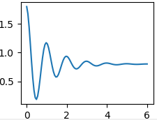
混入 # 综合练习1
import numpy as np
import matplotlib.pyplot as plt

x=np.linspace(0,6,100)
y=np.cos(2*np.pi*x)*np.exp(-x)+0.8

plt.plot(x,y)
plt.show()
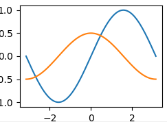
混入 # 综合练习2
import numpy as np
import matplotlib.pyplot as plt


x=np.linspace(-np.pi,np.pi,1000)
#print(x)


sin_y=np.sin(x)
#print(sin_y)

cos_y=np.cos(x)/2
#print(cos_y)

#绘制图
plt.plot(x,sin_y,x,cos_y)
#plt.plot(x,cos_y)

plt.show()
4、数组索引和切片
(1) 索引
1、 基本索引
数组对象[..., 页号, 行号, 列号],每个维度的索引规则和列表相同
import numpy as np
# 2页3行4列数组,24以内
a = np.arange(24).reshape(2,3,4)
print(a)
# [[[ 0  1  2  3]
#   [ 4  5  6  7]
#   [ 8  9 10 11]]
#
#  [[12 13 14 15]
#   [16 17 18 19]
#   [20 21 22 23]]]

# 基本索引练习, 第0页,第0页0行,倒数第一页倒数第2行第2列
print(a[0])  # 第0页
# [[12 13 14 15]
#  [16 17 18 19]
#  [20 21 22 23]]

print(a[0, 0])  # 第0页0行 [0 1 2 3]
print(a[-1, -2, 2])  # 倒数第 1页倒数第2行第2列 : 18
print(a[-2, -3, 3])  # 倒数第 2页倒数第3行第3列 : 3
2、 布尔索引
也叫掩码,是使用布尔类型的数组当做一个数组的索引,它可以使得我们可以从原数组中筛选出我们需要的数据。
import numpy as np
b = np.arange(24).reshape(6,4)
print(b)
# [[ 0  1  2  3]
#  [ 4  5  6  7]
#  [ 8  9 10 11]
#  [12 13 14 15]
#  [16 17 18 19]
#  [20 21 22 23]]

b_index = np.array([1,1,0,0,1,0], dtype = bool)
print(b_index) # [ True  True False False  True False]

print(".....布尔索引,一维索引......结果")
print(b[b_index])
# [[ 0  1  2  3]
#  [ 4  5  6  7]
#  [16 17 18 19]]
# 筛选数据,二维索引

import numpy as np
b =  np.arange(24).reshape(6,4)
print(b)
# [[ 0  1  2  3]
#  [ 4  5  6  7]
#  [ 8  9 10 11]
#  [12 13 14 15]
#  [16 17 18 19]
#  [20 21 22 23]]


b_index2 = b>11
print(b_index2)
# [[False False False False]
#  [False False False False]
#  [False False False False]
#  [ True  True  True  True]
#  [ True  True  True  True]
#  [ True  True  True  True]]

print(".....布尔索引,二维索引......结果")
print(b[b_index2])
# [12 13 14 15 16 17 18 19 20 21 22 23]
3、 花式索引
花式索引是使用整型数组(也可以是python中的列表)作为索引。
# 花式索引
import numpy as np
b = np.arange(24).reshape(6,4)
print(b)
# [[ 0  1  2  3]
#  [ 4  5  6  7]
#  [ 8  9 10 11]
#  [12 13 14 15]
#  [16 17 18 19]
#  [20 21 22 23]]

print(".....基本索引......结果")
print(b[0])  # 第一行: [0 1 2 3]
print(b[4,2]) # 第4行第2个(记得从0开始数):18

print(".....花式索引......结果")
print(b[[1,3,5]])  # 第1、3、5行
# [[ 4  5  6  7]
#  [12 13 14 15]
#  [20 21 22 23]]
print(b[[1,3,5]].T[1]) # 第1、3、5行转置后的第一行 [ 5 13 21]

print("...花式索引+基本索引...结果")
print(b[[1,3,5][0]]) # 第1、3、5行 的数列的 第一行 [4 5 6 7]

print("...花式索引 + 转置...结果")
c = b[[1,3,5]].T  # 第1、3、5行的转置
print(c)
# [[ 4 12 20]
#  [ 5 13 21]
#  [ 6 14 22]
#  [ 7 15 23]]
print(c[1]) # [ 5 13 21]
(2) 切片
数组对象[起始位置:终止位置:位置步长, ...] 如何理解:,... 这几个符号?
# 切片练习,二维数组
import numpy as np
a = np.arange(24).reshape(6,4)
print(a)
# [[ 0  1  2  3]
#  [ 4  5  6  7]
#  [ 8  9 10 11]
#  [12 13 14 15]
#  [16 17 18 19]
#  [20 21 22 23]]

print("...切片....行列...结果")
print(a[:, ::2]) # 切出全部,再切步长为 2
# [[ 0  2]
#  [ 4  6]
#  [ 8 10]
#  [12 14]
#  [16 18]
#  [20 22]]

print(a[::2])  # 切步长为 2
# [[ 0  1  2  3]
#  [ 8  9 10 11]
#  [16 17 18 19]]
# 切片练习,三维数组

import numpy as np
a =  np.arange(24).reshape(2,3,4)
print(a)
# [[[ 0  1  2  3]
#   [ 4  5  6  7]
#   [ 8  9 10 11]]

#  [[12 13 14 15]
#   [16 17 18 19]
#   [20 21 22 23]]]

print("...切片...页行列....结果1")
print(a[:,1:,::2])
# [[[ 4  6]
#   [ 8 10]]

#  [[16 18]
#   [20 22]]]

print(".....切片...页行....结果2")
print(a[:,1::2])
# [[[ 4  5  6  7]]

#  [[16 17 18 19]]]


 852
852


 被折叠的 条评论
为什么被折叠?
被折叠的 条评论
为什么被折叠?
 到【灌水乐园】发言


