神经网络——1.感知机

使用鸢尾花数据集中的其中花瓣长和花瓣宽数据，训练一个二分类的感知器，对0类iris和非0类iris进行二分类。

一、数据导入与预处理

import numpy as np
import pandas as pd
import matplotlib.pyplot as plt
from sklearn.datasets import load_iris
iris=load_iris()
df=pd.DataFrame(iris.data,columns=['sepal_length','sepal_width','petal_length','petal_weigh'])
df['label']=iris.target
df.describe()

#绘制散点图，观察数据特点
plt.scatter(df[df['label']==0]['sepal_length'],df[df['label']==0]['sepal_width'],marker='o',c='g')
plt.scatter(df[df['label']!=0]['sepal_length'],df[df['label']!=0]['sepal_width'],marker='x',c='r')
plt.xlabel('sepal_length')
plt.ylabel('sepal_width')
plt.legend(['0','else'])
plt.title('scatter of the 0-type iris and non-0-type iris')
plt.show()

df['new_label']=[1 if x==0 else -1 for x in df['label']]#发现可以用感知机根据两维数据划分0类和非0类，进行标签转换
df.head()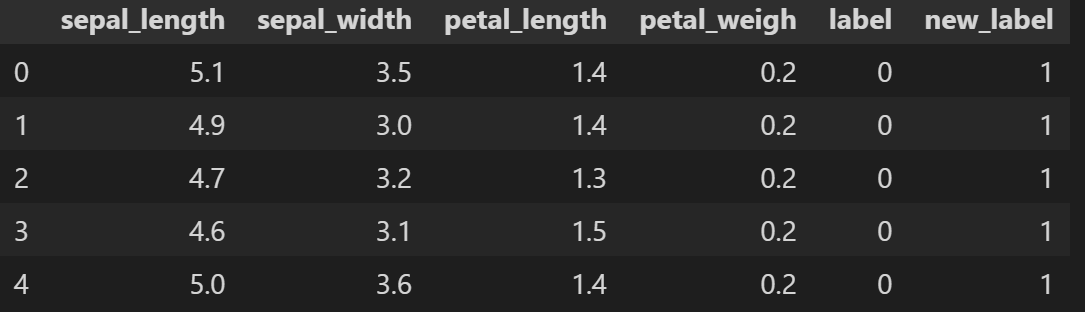

X=np.array(df[['sepal_length','sepal_width']])
y=np.array(df['new_label'])
y.resize(len(df),1)

二、模型定义

def hardlims(a):#激活函数
    return np.array([[1] if x>=0 else [-1] for x in a]) 
def predict(W,b,X):#感知器
    return hardlims(X@W+b)#X（n,2）,W(2,1),y(n,1)
def loss(W,b,X,y):#损失函数
    return -(y*(X@W+b)).sum()
W=np.array([[0],[0]])
b=0

三、训练

import random
import os
alpha=0.01
lossRec=[]
epoch=0
predicty=predict(W,b,X)
if not os.path.exists('img'):
    os.mkdir('img')
while((predicty==y).sum()!=y.size):
    diff=(predicty==y)#找出错分的序号
    row=[]
    for i in range(len(y)):
        if not diff[i]:
            row.append(i)
    unfity=y[row]
    unfitX=X[row]
    randindex=random.randint(0,unfity.size-1)#随机抽选一个错分的样本进行梯度下降
    W=(W.T+alpha*((unfity[randindex]*unfitX[randindex]))).T
    b=b+alpha*unfity[randindex]
    lossRec.append(loss(W,b,X,y))#计算loss
    epoch+=1
    predicty=predict(W,b,X)
    if epoch%10==0:#每10epoch输出loss并存图
        print('epoch%d loss:%.2f'%(epoch,lossRec[-1]))
        plt.figure(figsize=(10,10))
        plt.scatter(df[df['label']==0]['sepal_length'],df[df['label']==0]['sepal_width'],marker='o',c='g')
        plt.scatter(df[df['label']!=0]['sepal_length'],df[df['label']!=0]['sepal_width'],marker='x',c='r')
        plt.plot([[4],[5],[6],[7],[8]],-b/W[1]-np.array([[4],[5],[6],[7],[8]])*(W[0]/W[1]))
        plt.xlabel('sepal_length')
        plt.ylabel('sepal_width')
        plt.legend(['1','-1','the Preceptron'])
        plt.title('scatter of data and preceptron')
        plt.text(5,2,'epoch%d'%(epoch),color = "r",size=60)
        plt.xlim(4,8)
        plt.ylim(1.5,5.5)
        plt.savefig('img/%d.png'%(epoch))
        plt.close()

plt.figure(figsize=(20,10))
plt.plot(lossRec)
plt.title('loss figure')
plt.xlabel('epoch')
plt.ylabel('loss')
plt.xlim(0,1200)
plt.show()

四、可视化

#绘制散点图，观察数据特点
plt.figure(figsize=(10,10))
plt.scatter(df[df['label']==0]['sepal_length'],df[df['label']==0]['sepal_width'],marker='o',c='g')
plt.scatter(df[df['label']!=0]['sepal_length'],df[df['label']!=0]['sepal_width'],marker='x',c='r')
plt.plot([[4],[5],[6],[7],[8]],-b/W[1]-np.array([[4],[5],[6],[7],[8]])*(W[0]/W[1]))
plt.xlabel('sepal_length')
plt.ylabel('sepal_width')
plt.legend(['1','-1','the Preceptron'])
plt.title('scatter of data and preceptron')
plt.show()

import imageio
with imageio.get_writer(uri='preceptron.gif', mode='I', fps=5) as writer:
    for i in range(epoch//10):
        writer.append_data(imageio.imread('img/%d.png'%((i+1)*10)))
    writer.append_data(imageio.imread('img/final.png'))

Image("preceptron.gif")#显示