


#
# machine Learning with R cook book chapter 2
#
   # the Titanic data can be obtained from titanic package
   # or this link https://www.kaggle.com/c/titanic/data
   #
install.packages("titanic")
library(titanic)
train.data <- data(titanic_train)
write.csv(titanic_train,"D:/mlwrcbdataset/titanic_train.csv",row.names = TRUE)
#  load Titnic data set
train.data = read.csv(file="D:/mlwrcbdataset/titanic_train.csv", header = TRUE, sep = ",",na.strings = c("NA",""))
# check the loaded data with the str function:
str(train.data)
'data.frame': 891 obs. of 13 variables:
$ X : int 1 2 3 4 5 6 7 8 9 10 ...
$ PassengerId: int 1 2 3 4 5 6 7 8 9 10 ...
$ Survived : int 0 1 1 1 0 0 0 0 1 1 ...
$ Pclass : int 3 1 3 1 3 3 1 3 3 2 ...
$ Name : Factor w/ 891 levels "Abbing, Mr. Anthony",..: 109 191 358 277 16 559 520 629 417 581 ...
$ Sex : Factor w/ 2 levels "female","male": 2 1 1 1 2 2 2 2 1 1 ...
$ Age : num 22 38 26 35 35 NA 54 2 27 14 ...
$ SibSp : int 1 1 0 1 0 0 0 3 0 1 ...
$ Parch : int 0 0 0 0 0 0 0 1 2 0 ...
$ Ticket : Factor w/ 681 levels "110152","110413",..: 524 597 670 50 473 276 86 396 345 133 ...
$ Fare : num 7.25 71.28 7.92 53.1 8.05 ...
$ Cabin : Factor w/ 147 levels "A10","A14","A16",..: NA 82 NA 56 NA NA 130 NA NA NA ...
$ Embarked : Factor w/ 3 levels "C","Q","S": 3 1 3 3 3 2 3 3 3 1 ...
# transform the variable from the int numeric type to the factor categorical type
#  Survived (0 = No; 1 = Yes) and
#  Pclass (1 = 1st; 2 = 2nd; 3 = 3rd) are categorical variables
train.data$Survived = factor(train.data$Survived)
train.data$Pclass   = factor(train.data$Pclass)
str(train.data)$ X : int 1 2 3 4 5 6 7 8 9 10 ...
$ PassengerId: int 1 2 3 4 5 6 7 8 9 10 ...
$ Survived : Factor w/ 2 levels "0","1": 1 2 2 2 1 1 1 1 2 2 ...
$ Pclass : Factor w/ 3 levels "1","2","3": 3 1 3 1 3 3 1 3 3 2 ...
$ Name : Factor w/ 891 levels "Abbing, Mr. Anthony",..: 109 191 358 277 16 559 520 629 417 581 ...
$ Sex : Factor w/ 2 levels "female","male": 2 1 1 1 2 2 2 2 1 1 ...
$ Age : num 22 38 26 35 35 NA 54 2 27 14 ...
$ SibSp : int 1 1 0 1 0 0 0 3 0 1 ...
$ Parch : int 0 0 0 0 0 0 0 1 2 0 ...
$ Ticket : Factor w/ 681 levels "110152","110413",..: 524 597 670 50 473 276 86 396 345 133 ...
$ Fare : num 7.25 71.28 7.92 53.1 8.05 ...
$ Cabin : Factor w/ 147 levels "A10","A14","A16",..: NA 82 NA 56 NA NA 130 NA NA NA ...
$ Embarked : Factor w/ 3 levels "C","Q","S": 3 1 3 3 3 2 3 3 3 1 ...
# transform the variable from the int numeric type to the factor categorical type
#  Survived (0 = No; 1 = Yes) and
#  Pclass (1 = 1st; 2 = 2nd; 3 = 3rd) are categorical variables
train.data$Survived = factor(train.data$Survived)
train.data$Pclass   = factor(train.data$Pclass)
str(train.data)
# Detecting missing values
is.na(train.data$Age)
# how many missing values there are
sum(is.na(train.data$Age) == TRUE)# the percentage of missing values
sum(is.na(train.data$Age) == TRUE) / length(train.data$Age)# a percentage of the missing value of the attributes
sapply(train.data,function(df) {
sum(is.na(df)==TRUE)/length(df)
})0.000000000 0.000000000 0.000000000 0.000000000 0.000000000 0.000000000 0.198653199 0.000000000 0.000000000 0.000000000
Fare Cabin Embarked
0.000000000 0.771043771 0.002244669
   # use the missmap function to plot the missing value map:
install.packages("Amelia")
require(Amelia)
missmap(train.data,main="Missing Map")
# we can also use the interactive GUI of Amelia and AmeliaView,
# To start running AmeliaView, simply type AmeliaView() in the R Console
#
 # Imputing missing values
#
   # First, list the distribution of Port of Embarkation
table(train.data$Embarked, useNA = "always")168 77 644 2
   # Assign the two missing values to a more probable port
   # (that is, the most counted port), which is Southampton in this case:
train.data$Embarked[which(is.na(train.data$Embarked))] = 'S'
table(train.data$Embarked, useNA = "always")168 77 646 0
   # In order to discover the types of titles contained in the names of train.data, we
   # first tokenize train.data$Name by blank (a regular expression pattern as "\\s+"),
   # and then count the frequency of occurrence with the table function. After this, since
   # the name title often ends with a period, we use the regular expression to grep the
   # word containing the period. In the end, sort the table in decreasing order:
train.data$Name = as.character(train.data$Name)
table_words = table(unlist(strsplit(train.data$Name, "\\s+")))
sort(table_words [grep('\\.',names(table_words))], decreasing=TRUE)517 182 125 40 7 6 2 2 2 1 1 1
Jonkheer. L. Lady. Mme. Ms. Sir.
1 1 1 1 1 1
  # To obtain which title contains missing values, you can use str_match provided by
   # the stringr package to get a substring containing a period, then bind the column
   # together with cbind. Finally, by using the table function to acquire the statistics of
   # missing values, you can work on counting each title:
library(stringr)
tb = cbind(train.data$Age, str_match(train.data$Name, "[a-zA-Z]+\\."))
table(tb[is.na(tb[,1]),2])1 4 36 119 17
  # For a title containing a missing value, one way to impute data is to assign the mean
   # value for each title (not containing a missing value):
mean.mr   =  mean(train.data$Age[grepl(" Mr\\.",  train.data$Name) & !is.na(train.data$Age)])
mean.mrs  =  mean(train.data$Age[grepl(" Mrs\\.", train.data$Name) & !is.na(train.data$Age)])
mean.dr   =  mean(train.data$Age[grepl(" Dr\\.",  train.data$Name) & !is.na(train.data$Age)])
mean.miss =  mean(train.data$Age[grepl(" Miss\\.", train.data$Name) & !is.na(train.data$Age)])
mean.master = mean(train.data$Age[grepl(" Master\\.", train.data$Name) & !is.na(train.data$Age)])
   # Then, assign the missing value with the mean value of each title:
train.data$Age[grepl(" Mr\\.", train.data$Name) & is.na(train.data$Age)] = mean.mr
train.data$Age[grepl(" Mrs\\.", train.data$Name) & is.na(train.data$Age)] = mean.mrs
train.data$Age[grepl(" Dr\\.", train.data$Name) & is.na(train.data$Age)] = mean.dr
train.data$Age[grepl(" Miss\\.", train.data$Name) & is.na(train.data$Age)] = mean.miss
train.data$Age[grepl(" Master\\.", train.data$Name) & is.na(train.data$Age)] = mean.master
# Here we list the honorific entry from Wikipedia for your reference. According to it
# (http://en.wikipedia.org/wiki/English_honorific):
#
# Exploring and visualizing data
#
    # First, you can use a bar plot and histogram to generate descriptive statistics for each
    # attribute, starting with passenger survival:
barplot(table(train.data$Survived), main="Passenger Survival", names= c("Perished", "Survived"))
  # We can generate the bar plot of passenger class:
barplot(table(train.data$Pclass), main="Passenger Class",
        names= c("first", "second", "third"))
 # Next, we outline the gender data with the bar plot:
barplot(table(train.data$Sex), main="Passenger Gender")
# We then plot the histogram of the different ages with the hist function:
hist(train.data$Age, main="Passenger Age", xlab = "Age")
    # We can plot the bar plot of sibling passengers to get the following:
barplot(table(train.data$SibSp), main="Passenger Siblings")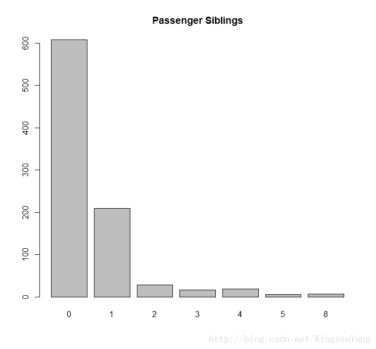
    # Next, we can get the distribution of the passenger parch:
barplot(table(train.data$Parch), main="Passenger Parch")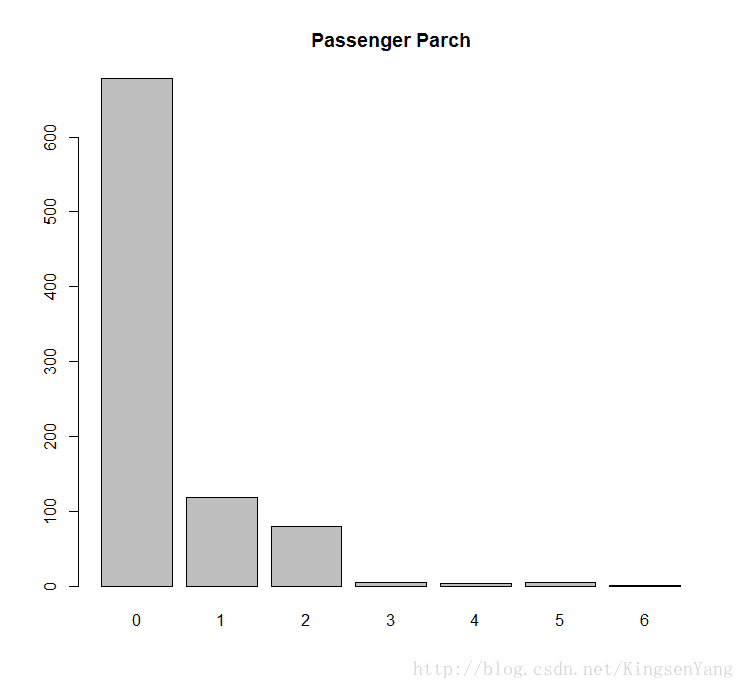
    # Next, we plot the histogram of the passenger fares:
hist(train.data$Fare, main="Passenger Fare", xlab = "Fare")
    # Finally, one can look at the port of embarkation:
barplot(table(train.data$Embarked), main="Port of Embarkation")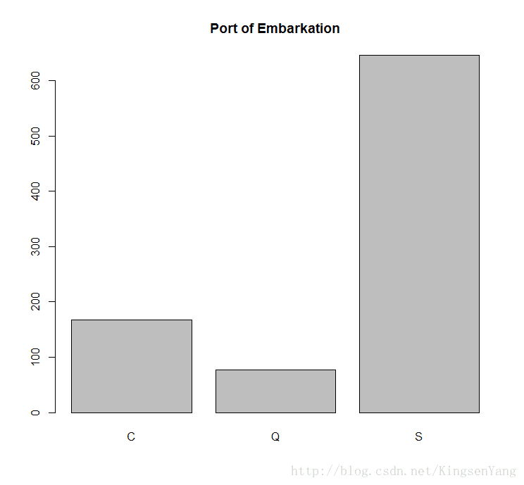
    # Use barplot to find out which gender is more likely to perish during shipwrecks
counts = table( train.data$Survived, train.data$Sex)
barplot(counts, col=c("darkblue","red"),
        legend = c("Perished", "Survived"),
        main = "Passenger Survival by Sex")
    # Next, we should examine whether the Pclass factor of each passenger
    # may affect the survival rate:
counts = table( train.data$Survived, train.data$Pclass)
barplot(counts, col=c("darkblue","red"),
        legend =c("Perished","Survived"),
        main= "Titanic Class Bar Plot" )
    # Next, we examine the gender composition of each Pclass:
counts = table( train.data$Sex, train.data$Pclass)
barplot(counts, col=c("darkblue","red"),
        legend = rownames(counts),
        main= "Passenger Gender by Class")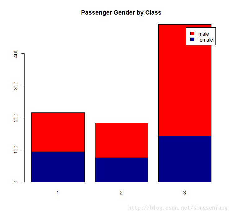
   # Furthermore, we examine the histogram of passenger ages
hist(train.data$Age[which(train.data$Survived == "0")],
     main= "Passenger Age Histogram",
     xlab="Age", ylab="Count", col ="blue",
     breaks=seq(0,80,by=2))
hist(train.data$Age[which(train.data$Survived == "1")],
     col  ="red", add = T,
     breaks=seq(0,80,by=2))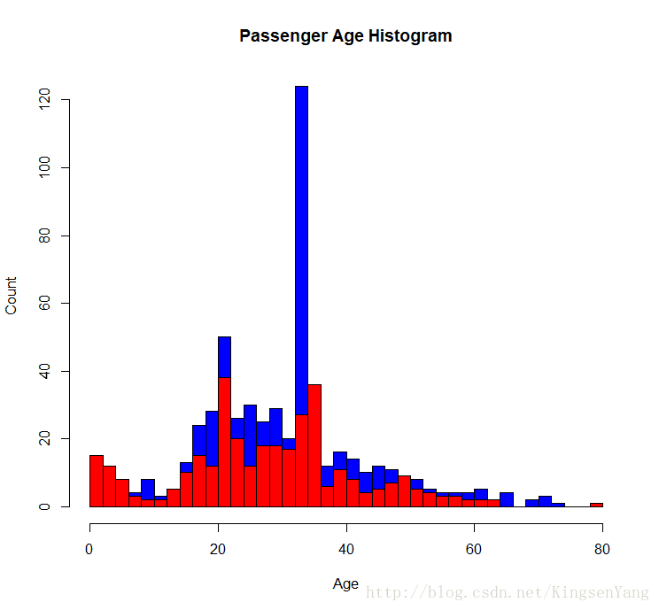
   # To examine more details about the relationship
   # between the age and survival rate, one can use a boxplot:
boxplot(train.data$Age ~ train.data$Survived,
        main="Passenger Survival by Age",
        xlab="Survived", ylab="Age")
# To categorize people with different ages into different groups, such as children (below
# 13), youths (13 to 19), adults (20 to 65), and senior citizens (above 65),
# execute the following commands:
train.child = train.data$Survived[train.data$Age < 13]
length(train.child[which(train.child == 1)] ) / length(train.child)train.youth = train.data$Survived[train.data$Age >= 15 & train.data$Age < 25]
length(train.youth[which(train.youth == 1)] ) / length(train.youth)train.adult = train.data$Survived[train.data$Age >= 20 & train.data$Age < 65]
length(train.adult[which(train.adult == 1)] ) / length(train.adult)train.senior = train.data$Survived[train.data$Age >= 65]
length(train.senior[which(train.senior == 1)] ) / length(train.senior) # Apart from using bar plots, histograms, and boxplots to visualize data, one can also apply
# mosaicplot in the vcd package to examine the relationship between multiple categorical
# variables. For example, when we examine the relationship between the Survived and
# Pclass variables, the application is performed as follows:
mosaicplot(train.data$Pclass ~ train.data$Survived,
main="Passenger Survival Class", color=TRUE,
xlab="Pclass", ylab="Survived")
#
# Predicting passenger survival with a decision tree
#
   # First, we construct a data split split.data function
split.data = function(data, p = 0.7, s = 666){
   set.seed(s)
   index = sample(1:dim(data)[1])
   train = data[index[1:floor(dim(data)[1] * p)], ]
   test = data[index[((ceiling(dim(data)[1] * p)) + 1):dim(data)[1]], ]
   return(list(train = train, test = test))
   }
    # Then, we split the data, with 70 percent assigned to the training dataset and the
    # remaining 30 percent for the testing dataset:
allset= split.data(train.data, p = 0.7)
trainset = allset$train
testset = allset$test
    # For the condition tree, one has to use the ctree function from the party package;
    # therefore, we install and load the party package:
install.packages('party')
require('party')
    # We then use Survived as a label to generate the prediction model in use. After that,
    # we assign the classification tree model into the train.ctree variable:
train.ctree = ctree(Survived ~ Pclass + Sex + Age + SibSp + Fare
                     +Parch + Embarked, data=trainset)
train.ctreeResponse: Survived
Inputs: Pclass, Sex, Age, SibSp, Fare, Parch, Embarked
Number of observations: 623
1) Sex == {male}; criterion = 1, statistic = 173.672
2) Pclass == {2, 3}; criterion = 1, statistic = 30.951
3) Age <= 9; criterion = 0.993, statistic = 10.923
4) SibSp <= 1; criterion = 0.999, statistic = 14.856
5)* weights = 10
4) SibSp > 1
6)* weights = 13
3) Age > 9
7)* weights = 280
2) Pclass == {1}
8)* weights = 87
1) Sex == {female}
9) Pclass == {1, 2}; criterion = 1, statistic = 59.504
10)* weights = 125
9) Pclass == {3}
11) Fare <= 23.25; criterion = 0.997, statistic = 12.456
12)* weights = 85
11) Fare > 23.25
13)* weights = 23
    # We use a plot function to plot the tree:
 plot(train.ctree, main="Conditional inference tree of Titanic Dataset")
    # There is a similar decision tree based package, named rpart. The difference between party
    # and rpart is that ctree in the party package avoids the following variable selection bias of
    # rpart and ctree in the party package, tending to select variables that have many possible
    # splits or many missing values. Unlike the others, ctree uses a significance testing procedure
    # in order to select variables, instead of selecting the variable that maximizes an information
    # measure.
#
# Validating the power of prediction with a confusion matrix
#
    # We start using the constructed train.ctree model to predict the survival of the
    # testing set:
ctree.predict = predict(train.ctree, testset)
    # First, we install the caret package, and then load it:
install.packages("caret")
require(caret)
    # After loading caret, one can use a confusion matrix to generate the statistics of the
    # output matrix:
confusionMatrix(ctree.predict, testset$Survived)Reference
Prediction 0 1
0 160 23
1 16 68
Accuracy : 0.8539
95% CI : (0.8058, 0.894)
No Information Rate : 0.6592
P-Value [Acc > NIR] : 5.347e-13
Kappa : 0.6688
Mcnemar's Test P-Value : 0.3367
Sensitivity : 0.9091
Specificity : 0.7473
Pos Pred Value : 0.8743
Neg Pred Value : 0.8095
Prevalence : 0.6592
Detection Rate : 0.5993
Detection Prevalence : 0.6854
Balanced Accuracy : 0.8282
'Positive' Class : 0
 # Assessing performance with the ROC curve
    # Prepare the probability matrix:
train.ctree.pred = predict(train.ctree, testset)
train.ctree.prob = 1- unlist(treeresponse(train.ctree,testset), use.names=F)[seq(1,nrow(testset)*2,2)]
    # Install and load the ROCR package:
install.packages("ROCR")
require(ROCR)
    # Create an ROCR prediction object from probabilities
train.ctree.prob.rocr = prediction(train.ctree.prob,testset$Survived)
    # Prepare the ROCR performance object for the ROC curve (tpr=true positive
    # rate, fpr=false positive rate) and the area under curve (AUC):
train.ctree.perf = performance(train.ctree.prob.rocr,"tpr","fpr")
train.ctree.auc.perf = performance(train.ctree.prob.rocr,
                                   measure = "auc", x.measure = "cutoff")
    # Plot the ROC curve, with colorize as TRUE, and put AUC as the title:
plot(train.ctree.perf, col=2,colorize=T,
     main=paste("AUC:", train.ctree.auc.perf@y.values))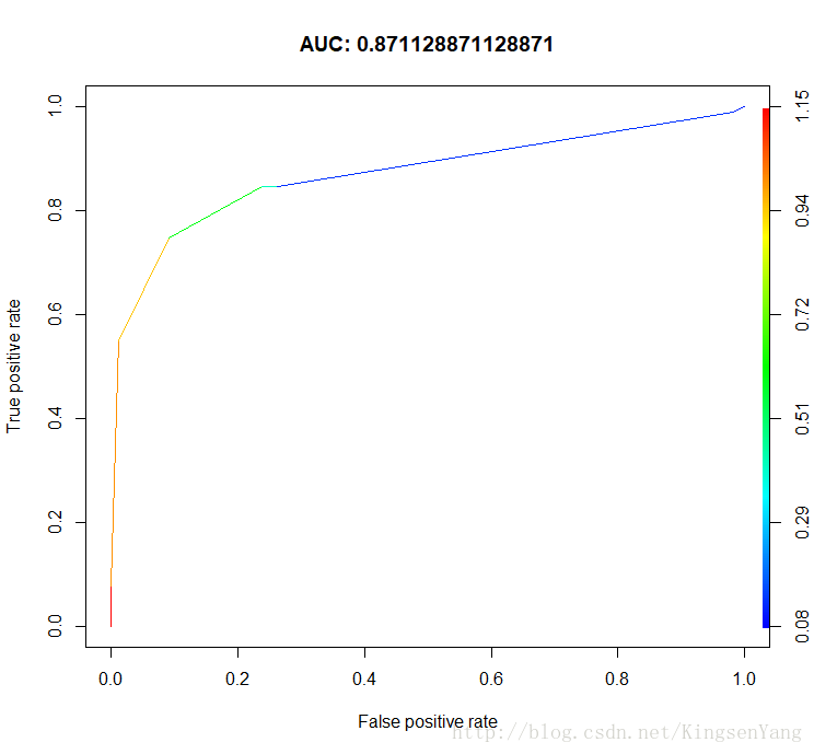


 1250
1250


 被折叠的 条评论
为什么被折叠?
被折叠的 条评论
为什么被折叠?
 到【灌水乐园】发言


