


目录
一、预处理流程回顾
- 导入库
- 读取数据查看数据信息--理解数据
- 缺失值处理
- 异常值处理
- 离散值处理
- 删除无用列
- 划分数据集
- 特征工程
- 模型训练
- 模型评估
- 模型保存
- 模型预测
1. 导入所需要的包
这里其实是写完后一起整理到这里的
import pandas as pd
import pandas as pd    #用于数据处理和分析,可处理表格数据。
import numpy as np     #用于数值计算,提供了高效的数组操作。
import matplotlib.pyplot as plt    #用于绘制各种类型的图表
import seaborn as sns   #基于matplotlib的高级绘图库,能绘制更美观的统计图形。

 # 设置中文字体(解决中文显示问题)
plt.rcParams['font.sans-serif'] = ['SimHei']  # Windows系统常用黑体字体
plt.rcParams['axes.unicode_minus'] = False    # 正常显示负号
2. 查看数据信息
data = pd.read_csv('data.csv')    #读取数据
print("数据基本信息:")
data.info()
print("\n数据前5行预览:")
print(data.head())
数据基本信息:
<class 'pandas.core.frame.DataFrame'>
RangeIndex: 7500 entries, 0 to 7499
Data columns (total 18 columns):
# Column Non-Null Count Dtype
--- ------ -------------- -----
0 Id 7500 non-null int64
1 Home Ownership 7500 non-null object
2 Annual Income 5943 non-null float64
3 Years in current job 7129 non-null object
4 Tax Liens 7500 non-null float64
5 Number of Open Accounts 7500 non-null float64
6 Years of Credit History 7500 non-null float64
7 Maximum Open Credit 7500 non-null float64
8 Number of Credit Problems 7500 non-null float64
9 Months since last delinquent 3419 non-null float64
10 Bankruptcies 7486 non-null float64
11 Purpose 7500 non-null object
12 Term 7500 non-null object
13 Current Loan Amount 7500 non-null float64
14 Current Credit Balance 7500 non-null float64
15 Monthly Debt 7500 non-null float64
16 Credit Score 5943 non-null float64
17 Credit Default 7500 non-null int64
dtypes: float64(12), int64(2), object(4)
memory usage: 1.0+ MB
数据前5行预览:
Id Home Ownership Annual Income Years in current job Tax Liens \
0 0 Own Home 482087.0 NaN 0.0
1 1 Own Home 1025487.0 10+ years 0.0
2 2 Home Mortgage 751412.0 8 years 0.0
3 3 Own Home 805068.0 6 years 0.0
4 4 Rent 776264.0 8 years 0.0
Number of Open Accounts Years of Credit History Maximum Open Credit \
0 11.0 26.3 685960.0
1 15.0 15.3 1181730.0
2 11.0 35.0 1182434.0
3 8.0 22.5 147400.0
4 13.0 13.6 385836.0
Number of Credit Problems Months since last delinquent Bankruptcies \
0 1.0 NaN 1.0
1 0.0 NaN 0.0
2 0.0 NaN 0.0
3 1.0 NaN 1.0
4 1.0 NaN 0.0
Purpose Term Current Loan Amount \
0 debt consolidation Short Term 99999999.0
1 debt consolidation Long Term 264968.0
2 debt consolidation Short Term 99999999.0
3 debt consolidation Short Term 121396.0
4 debt consolidation Short Term 125840.0
Current Credit Balance Monthly Debt Credit Score Credit Default
0 47386.0 7914.0 749.0 0
1 394972.0 18373.0 737.0 1
2 308389.0 13651.0 742.0 0
3 95855.0 11338.0 694.0 0
4 93309.0 7180.0 719.0 0
以下是对该数据集进行预处理的步骤及顺序:
一共有17个特征,分别处理
- 缺失值处理
- Annual Income:有5943个非空值,存在缺失值。可以考虑使用均值填充、中位数填充或者基于其他相关特征进行回归预测填充。例如,如果“Home Ownership”和“Annual Income”有一定相关性,可根据不同房屋所有权类型的平均收入来填充缺失值。
- Years in current job:7129个非空值,存在缺失值。由于是对象类型,可能需要先将其转换为合适的数值类型再进行处理。比如将“10+ years”转换为10,“8 years”转换为8等,然后再用众数或中位数填充缺失值。
- Months since last delinquent:只有3419个非空值,缺失值较多。若该特征对目标变量影响较大,可尝试用多重填补法等较为复杂的方法进行填充;若影响较小,也可直接删除含有缺失值的行,但要注意可能会导致数据量损失较大。
- Credit Score:5943个非空值,存在缺失值。可参照“Annual Income”的处理方式,根据与其他特征的相关性来选择合适的填充方法。
- 数据类型转换
- Years in current job:将其从对象类型转换为数值类型,方便后续的计算和模型处理。
- Home Ownership、Purpose、Term:这些对象类型的特征可以进行独热编码或标签编码。如果特征的类别数较少且没有明显的顺序关系,独热编码较为合适;如果有一定的顺序关系,如“Term”的“Short Term”和“Long Term”,可以考虑标签编码。
- 异常值处理
- 对于数值型特征,如“Annual Income”“Current Loan Amount”等,可以通过箱线图等方法检测异常值。如果存在异常值,需根据实际情况决定是否进行处理。若是数据录入错误等原因导致的异常值,可以进行修正或删除;若是真实存在的极端值,可能需要保留,但在某些模型中可能需要进行特殊处理,如采用稳健的统计方法或对数据进行变换。
- 特征缩放
- 对数值型特征进行特征缩放,将其缩放到相同的尺度,以避免某些特征因数值较大而在模型中占据主导地位。常用的方法有Min - Max标准化和Z - score标准化。例如,“Annual Income”“Years of Credit History”“Credit Score”等特征的取值范围差异较大,可通过特征缩放将它们的取值范围统一到[0, 1]或均值为0、标准差为1的分布上。
- 特征工程
- 衍生新特征:根据已有特征创建新的特征,可能会对模型性能有提升。例如,可以计算“Debt - to - Income Ratio”(负债收入比),即“Monthly Debt”与“Annual Income”的比值,来反映客户的债务负担情况。
- 特征选择:通过相关性分析等方法,选择与目标变量“Credit Default”相关性较高的特征,去除相关性较低或冗余的特征,以降低模型的复杂度和过拟合的风险。
在实际操作中,需要先进行缺失值处理,然后进行数据类型转换,接着处理异常值,再进行特征缩放,最后进行特征工程。这样的顺序可以保证数据在预处理过程中的一致性和有效性,为后续的机器学习模型训练提供高质量的数据。
3. 首先处理object变量
因为最后的输入都是数值类型,所以先给字符串变量处理了
# 先筛选字符串变量
discrete_features = data.select_dtypes(include=['object']).columns.tolist()
discrete_features
['Home Ownership', 'Years in current job', 'Purpose', 'Term']
# 依次查看内容
for feature in discrete_features:
    print(f"\n{feature}的唯一值:")
    print(data[feature].value_counts())
Home Ownership的唯一值: Home Mortgage 3637 Rent 3204 Own Home 647 Have Mortgage 12 Name: Home Ownership, dtype: int64 Years in current job的唯一值: 10+ years 2332 2 years 705 3 years 620 < 1 year 563 5 years 516 1 year 504 4 years 469 6 years 426 7 years 396 8 years 339 9 years 259 Name: Years in current job, dtype: int64 Purpose的唯一值: debt consolidation 5944 other 665 home improvements 412 business loan 129 buy a car 96 medical bills 71 major purchase 40 take a trip 37 buy house 34 small business 26 wedding 15 moving 11 educational expenses 10 vacation 8 renewable energy 2 Name: Purpose, dtype: int64 Term的唯一值: Short Term 5556 Long Term 1944 Name: Term, dtype: int64
Home Ownership需要标签编码。
- 住房抵押贷款:3637 这个是有房贷,有房子
- 租房:3204 没房子
- 拥有自有住房:647 这个没贷款,有房子
- 有贷款:12 这个是有其他贷款,有房子,没房贷
- 名称:房屋所有权,数据类型:int64
按照贷款严重程度(抗风险能力),依次是:自有住房 < 租房 < 有其他贷款 < 住房抵押贷款
所以按照这个逻辑来进行编码
Years in current job 做标签编码
Purpose做独热编码
Term直接做0-1映射即可,二分类问题,处理后更改自己的名字为1的类别
# Home Ownership 标签编码
home_ownership_mapping = {
    'Own Home': 1,
    'Rent': 2,
    'Have Mortgage': 3,
    'Home Mortgage': 4
}
data['Home Ownership'] = data['Home Ownership'].map(home_ownership_mapping)

# Years in current job 标签编码
years_in_job_mapping = {
    '< 1 year': 1,
    '1 year': 2,
    '2 years': 3,
    '3 years': 4,
    '4 years': 5,
    '5 years': 6,
    '6 years': 7,
    '7 years': 8,
    '8 years': 9,
    '9 years': 10,
    '10+ years': 11
}
data['Years in current job'] = data['Years in current job'].map(years_in_job_mapping)

# Purpose 独热编码,记得需要将bool类型转换为数值
data = pd.get_dummies(data, columns=['Purpose'])
data2 = pd.read_csv("data.csv") # 重新读取数据,用来做列名对比
list_final = [] # 新建一个空列表,用于存放独热编码后新增的特征名
for i in data.columns:
    if i not in data2.columns:
       list_final.append(i) # 这里打印出来的就是独热编码后的特征名
for i in list_final:
    data[i] = data[i].astype(int) # 这里的i就是独热编码后的特征名


# Term 0 - 1 映射
term_mapping = {
    'Short Term': 0,
    'Long Term': 1
}
data['Term'] = data['Term'].map(term_mapping)
data.rename(columns={'Term': 'Long Term'}, inplace=True) # 重命名列
4. 处理数值型对象
4.1 缺失值填补
continuous_features = data.select_dtypes(include=['int64', 'float64']).columns.tolist()  #把筛选出来的列名转换成列表

 # 连续特征用中位数补全
for feature in continuous_features:
    mode_value = data[feature].mode()[0]            #获取该列的众数。
    data[feature].fillna(mode_value, inplace=True)          #用众数填充该列的缺失值,inplace=True表示直接在原数据上修改。
4.2 异常值处理
异常值一般不处理,或者结合对照试验处理和不处理都尝试下
data.info() #查看数据基本信息<class 'pandas.core.frame.DataFrame'> RangeIndex: 7500 entries, 0 to 7499 Data columns (total 32 columns): # Column Non-Null Count Dtype --- ------ -------------- ----- 0 Id 7500 non-null int64 1 Home Ownership 7500 non-null int64 2 Annual Income 7500 non-null float64 3 Years in current job 7500 non-null float64 4 Tax Liens 7500 non-null float64 5 Number of Open Accounts 7500 non-null float64 6 Years of Credit History 7500 non-null float64 7 Maximum Open Credit 7500 non-null float64 8 Number of Credit Problems 7500 non-null float64 9 Months since last delinquent 7500 non-null float64 10 Bankruptcies 7500 non-null float64 11 Long Term 7500 non-null int64 12 Current Loan Amount 7500 non-null float64 13 Current Credit Balance 7500 non-null float64 14 Monthly Debt 7500 non-null float64 15 Credit Score 7500 non-null float64 16 Credit Default 7500 non-null int64 17 Purpose_business loan 7500 non-null int32 18 Purpose_buy a car 7500 non-null int32 19 Purpose_buy house 7500 non-null int32 20 Purpose_debt consolidation 7500 non-null int32 21 Purpose_educational expenses 7500 non-null int32 22 Purpose_home improvements 7500 non-null int32 23 Purpose_major purchase 7500 non-null int32 24 Purpose_medical bills 7500 non-null int32 25 Purpose_moving 7500 non-null int32 26 Purpose_other 7500 non-null int32 27 Purpose_renewable energy 7500 non-null int32 28 Purpose_small business 7500 non-null int32 29 Purpose_take a trip 7500 non-null int32 30 Purpose_vacation 7500 non-null int32 31 Purpose_wedding 7500 non-null int32 dtypes: float64(13), int32(15), int64(4) memory usage: 1.4 MB
此时数据没有缺失值
5. 可视化分析
这部分比较随意,根据自己的需要来绘制图像,作为描述性统计部分,向他人介绍你的数据分布。
二、机器学习建模与评估
首先进行数据划分,这里我们先不调参,所以只需要划分一次即可。
1. 数据划分
# 划分训练集和测试机
from sklearn.model_selection import train_test_split
X = data.drop(['Credit Default'], axis=1)  # 特征,axis=1表示按列删除
y = data['Credit Default']  # 标签
X_train, X_test, y_train, y_test = train_test_split(X, y, test_size=0.2, random_state=42)  # 划分数据集,20%作为测试集,随机种子为42
# 训练集和测试集的形状
print(f"训练集形状: {X_train.shape}, 测试集形状: {X_test.shape}")  # 打印训练集和测试集的形状
训练集形状: (6000, 31), 测试集形状: (1500, 31)
2. 模型训练与评估
三行经典代码
- 模型实例化
- 模型训练(代入训练集)
- 模型预测 (代入测试集)
测试集的预测值和测试集的真实值进行对比,得到混淆矩阵
-
基于混淆矩阵,计算准确率、召回率、F1值,这些都是固定阈值的评估指标
-
AUC是基于不同阈值得到不同的混淆矩阵,然后计算每个阈值对应FPR和TPR,讲这些点连成线,最后求曲线下的面积,得到AUC值
# #安装xgboost库
# !pip install xgboost -i https://pypi.tuna.tsinghua.edu.cn/simple/
# #安装lightgbm库
# !pip install lightgbm  -i https://pypi.tuna.tsinghua.edu.cn/simple/
# #安装catboost库
# !pip install catboost -i https://pypi.tuna.tsinghua.edu.cn/simple/
from sklearn.svm import SVC #支持向量机分类器
from sklearn.neighbors import KNeighborsClassifier #K近邻分类器
from sklearn.linear_model import LogisticRegression #逻辑回归分类器
import xgboost as xgb #XGBoost分类器
import lightgbm as lgb #LightGBM分类器
from sklearn.ensemble import RandomForestClassifier #随机森林分类器
from catboost import CatBoostClassifier #CatBoost分类器
from sklearn.tree import DecisionTreeClassifier #决策树分类器
from sklearn.naive_bayes import GaussianNB #高斯朴素贝叶斯分类器
from sklearn.metrics import accuracy_score, precision_score, recall_score, f1_score # 用于评估分类器性能的指标
from sklearn.metrics import classification_report, confusion_matrix #用于生成分类报告和混淆矩阵
import warnings #用于忽略警告信息
warnings.filterwarnings("ignore") # 忽略所有警告信息
# SVM
svm_model = SVC(random_state=42)
svm_model.fit(X_train, y_train)
svm_pred = svm_model.predict(X_test)
print("\nSVM 分类报告:")
print(classification_report(y_test, svm_pred)) # 打印分类报告
print("SVM 混淆矩阵:")
print(confusion_matrix(y_test, svm_pred)) # 打印混淆矩阵
# 计算 SVM 评估指标,这些指标默认计算正类的性能
svm_accuracy = accuracy_score(y_test, svm_pred)
svm_precision = precision_score(y_test, svm_pred)
svm_recall = recall_score(y_test, svm_pred)
svm_f1 = f1_score(y_test, svm_pred)
print("SVM 模型评估指标:")
print(f"准确率: {svm_accuracy:.4f}")
print(f"精确率: {svm_precision:.4f}")
print(f"召回率: {svm_recall:.4f}")
print(f"F1 值: {svm_f1:.4f}")SVM 分类报告:
precision recall f1-score support
0 0.71 1.00 0.83 1059
1 0.00 0.00 0.00 441
accuracy 0.71 1500
macro avg 0.35 0.50 0.41 1500
weighted avg 0.50 0.71 0.58 1500
SVM 混淆矩阵:
[[1059 0]
[ 441 0]]
SVM 模型评估指标:
准确率: 0.7060
精确率: 0.0000
召回率: 0.0000
F1 值: 0.0000
classification_report它会生成所有类别的指标
准确率(Accuracy)是一个全局指标,衡量所有类别预测正确的比例 (TP + TN) / (TP + TN + FP + FN)。它不区分正负类,所以它只有一个值,不区分类别
单独调用的 precision_score, recall_score, f1_score 在二分类中默认只计算正类(标签 1)的性能。由于模型从未成功预测出类别 1(TP=0),所以这些指标对类别 1 来说都是 0。
# KNN
knn_model = KNeighborsClassifier()
knn_model.fit(X_train, y_train)
knn_pred = knn_model.predict(X_test)

print("\nKNN 分类报告:")
print(classification_report(y_test, knn_pred))
print("KNN 混淆矩阵:")
print(confusion_matrix(y_test, knn_pred))

knn_accuracy = accuracy_score(y_test, knn_pred)
knn_precision = precision_score(y_test, knn_pred)
knn_recall = recall_score(y_test, knn_pred)
knn_f1 = f1_score(y_test, knn_pred)
print("KNN 模型评估指标:")
print(f"准确率: {knn_accuracy:.4f}")
print(f"精确率: {knn_precision:.4f}")
print(f"召回率: {knn_recall:.4f}")
print(f"F1 值: {knn_f1:.4f}")
KNN 分类报告:
precision recall f1-score support
0 0.73 0.86 0.79 1059
1 0.41 0.24 0.30 441
accuracy 0.68 1500
macro avg 0.57 0.55 0.54 1500
weighted avg 0.64 0.68 0.65 1500
KNN 混淆矩阵:
[[908 151]
[336 105]]
KNN 模型评估指标:
准确率: 0.6753
精确率: 0.4102
召回率: 0.2381
F1 值: 0.3013
# 逻辑回归
logreg_model = LogisticRegression(random_state=42)
logreg_model.fit(X_train, y_train)
logreg_pred = logreg_model.predict(X_test)

print("\n逻辑回归 分类报告:")
print(classification_report(y_test, logreg_pred))
print("逻辑回归 混淆矩阵:")
print(confusion_matrix(y_test, logreg_pred))

logreg_accuracy = accuracy_score(y_test, logreg_pred)
logreg_precision = precision_score(y_test, logreg_pred)
logreg_recall = recall_score(y_test, logreg_pred)
logreg_f1 = f1_score(y_test, logreg_pred)
print("逻辑回归 模型评估指标:")
print(f"准确率: {logreg_accuracy:.4f}")
print(f"精确率: {logreg_precision:.4f}")
print(f"召回率: {logreg_recall:.4f}")
print(f"F1 值: {logreg_f1:.4f}")
逻辑回归 分类报告:
precision recall f1-score support
0 0.75 0.99 0.85 1059
1 0.86 0.20 0.33 441
accuracy 0.76 1500
macro avg 0.80 0.59 0.59 1500
weighted avg 0.78 0.76 0.70 1500
逻辑回归 混淆矩阵:
[[1044 15]
[ 351 90]]
逻辑回归 模型评估指标:
准确率: 0.7560
精确率: 0.8571
召回率: 0.2041
F1 值: 0.3297
# 朴素贝叶斯
nb_model = GaussianNB()
nb_model.fit(X_train, y_train)
nb_pred = nb_model.predict(X_test)

print("\n朴素贝叶斯 分类报告:")
print(classification_report(y_test, nb_pred))
print("朴素贝叶斯 混淆矩阵:")
print(confusion_matrix(y_test, nb_pred))

nb_accuracy = accuracy_score(y_test, nb_pred)
nb_precision = precision_score(y_test, nb_pred)
nb_recall = recall_score(y_test, nb_pred)
nb_f1 = f1_score(y_test, nb_pred)
print("朴素贝叶斯 模型评估指标:")
print(f"准确率: {nb_accuracy:.4f}")
print(f"精确率: {nb_precision:.4f}")
print(f"召回率: {nb_recall:.4f}")
print(f"F1 值: {nb_f1:.4f}")
朴素贝叶斯 分类报告:
precision recall f1-score support
0 0.98 0.19 0.32 1059
1 0.34 0.99 0.50 441
accuracy 0.43 1500
macro avg 0.66 0.59 0.41 1500
weighted avg 0.79 0.43 0.38 1500
朴素贝叶斯 混淆矩阵:
[[204 855]
[ 5 436]]
朴素贝叶斯 模型评估指标:
准确率: 0.4267
精确率: 0.3377
召回率: 0.9887
F1 值: 0.5035
# 决策树
dt_model = DecisionTreeClassifier(random_state=42)
dt_model.fit(X_train, y_train)
dt_pred = dt_model.predict(X_test)

print("\n决策树 分类报告:")
print(classification_report(y_test, dt_pred))
print("决策树 混淆矩阵:")
print(confusion_matrix(y_test, dt_pred))

dt_accuracy = accuracy_score(y_test, dt_pred)
dt_precision = precision_score(y_test, dt_pred)
dt_recall = recall_score(y_test, dt_pred)
dt_f1 = f1_score(y_test, dt_pred)
print("决策树 模型评估指标:")
print(f"准确率: {dt_accuracy:.4f}")
print(f"精确率: {dt_precision:.4f}")
print(f"召回率: {dt_recall:.4f}")
print(f"F1 值: {dt_f1:.4f}")
决策树 分类报告:
precision recall f1-score support
0 0.79 0.75 0.77 1059
1 0.46 0.51 0.48 441
accuracy 0.68 1500
macro avg 0.62 0.63 0.62 1500
weighted avg 0.69 0.68 0.68 1500
决策树 混淆矩阵:
[[791 268]
[216 225]]
决策树 模型评估指标:
准确率: 0.6773
精确率: 0.4564
召回率: 0.5102
F1 值: 0.4818
# 随机森林
rf_model = RandomForestClassifier(random_state=42)
rf_model.fit(X_train, y_train)
rf_pred = rf_model.predict(X_test)

print("\n随机森林 分类报告:")
print(classification_report(y_test, rf_pred))
print("随机森林 混淆矩阵:")
print(confusion_matrix(y_test, rf_pred))

rf_accuracy = accuracy_score(y_test, rf_pred)
rf_precision = precision_score(y_test, rf_pred)
rf_recall = recall_score(y_test, rf_pred)
rf_f1 = f1_score(y_test, rf_pred)
print("随机森林 模型评估指标:")
print(f"准确率: {rf_accuracy:.4f}")
print(f"精确率: {rf_precision:.4f}")
print(f"召回率: {rf_recall:.4f}")
print(f"F1 值: {rf_f1:.4f}")
随机森林 分类报告:
precision recall f1-score support
0 0.77 0.97 0.86 1059
1 0.79 0.30 0.43 441
accuracy 0.77 1500
macro avg 0.78 0.63 0.64 1500
weighted avg 0.77 0.77 0.73 1500
随机森林 混淆矩阵:
[[1023 36]
[ 309 132]]
随机森林 模型评估指标:
准确率: 0.7700
精确率: 0.7857
召回率: 0.2993
F1 值: 0.4335
# XGBoost
xgb_model = xgb.XGBClassifier(random_state=42)
xgb_model.fit(X_train, y_train)
xgb_pred = xgb_model.predict(X_test)

print("\nXGBoost 分类报告:")
print(classification_report(y_test, xgb_pred))
print("XGBoost 混淆矩阵:")
print(confusion_matrix(y_test, xgb_pred))

xgb_accuracy = accuracy_score(y_test, xgb_pred)
xgb_precision = precision_score(y_test, xgb_pred)
xgb_recall = recall_score(y_test, xgb_pred)
xgb_f1 = f1_score(y_test, xgb_pred)
print("XGBoost 模型评估指标:")
print(f"准确率: {xgb_accuracy:.4f}")
print(f"精确率: {xgb_precision:.4f}")
print(f"召回率: {xgb_recall:.4f}")
print(f"F1 值: {xgb_f1:.4f}")
XGBoost 分类报告:
precision recall f1-score support
0 0.77 0.91 0.84 1059
1 0.62 0.37 0.46 441
accuracy 0.75 1500
macro avg 0.70 0.64 0.65 1500
weighted avg 0.73 0.75 0.72 1500
XGBoost 混淆矩阵:
[[960 99]
[280 161]]
XGBoost 模型评估指标:
准确率: 0.7473
精确率: 0.6192
召回率: 0.3651
F1 值: 0.4593
# LightGBM
lgb_model = lgb.LGBMClassifier(random_state=42)
lgb_model.fit(X_train, y_train)
lgb_pred = lgb_model.predict(X_test)

print("\nLightGBM 分类报告:")
print(classification_report(y_test, lgb_pred))
print("LightGBM 混淆矩阵:")
print(confusion_matrix(y_test, lgb_pred))

lgb_accuracy = accuracy_score(y_test, lgb_pred)
lgb_precision = precision_score(y_test, lgb_pred)
lgb_recall = recall_score(y_test, lgb_pred)
lgb_f1 = f1_score(y_test, lgb_pred)
print("LightGBM 模型评估指标:")
print(f"准确率: {lgb_accuracy:.4f}")
print(f"精确率: {lgb_precision:.4f}")
print(f"召回率: {lgb_recall:.4f}")
print(f"F1 值: {lgb_f1:.4f}")
[LightGBM] [Warning] Found whitespace in feature_names, replace with underlines
[LightGBM] [Info] Number of positive: 1672, number of negative: 4328
[LightGBM] [Info] Auto-choosing row-wise multi-threading, the overhead of testing was 0.001826 seconds.
You can set `force_row_wise=true` to remove the overhead.
And if memory is not enough, you can set `force_col_wise=true`.
[LightGBM] [Info] Total Bins 2160
[LightGBM] [Info] Number of data points in the train set: 6000, number of used features: 26
[LightGBM] [Info] [binary:BoostFromScore]: pavg=0.278667 -> initscore=-0.951085
[LightGBM] [Info] Start training from score -0.951085
LightGBM 分类报告:
precision recall f1-score support
0 0.78 0.94 0.85 1059
1 0.70 0.36 0.47 441
accuracy 0.77 1500
macro avg 0.74 0.65 0.66 1500
weighted avg 0.75 0.77 0.74 1500
LightGBM 混淆矩阵:
[[992 67]
[284 157]]
LightGBM 模型评估指标:
准确率: 0.7660
精确率: 0.7009
召回率: 0.3560
F1 值: 0.4722
| 模型名称 | 准确率 | 精确率(正类) | 召回率(正类) | F1值(正类) | 精确率(负类) | 召回率(负类) | F1值(负类) |
|---|---|---|---|---|---|---|---|
| SVM | 0.7060 | 0.0000 | 0.0000 | 0.0000 | 0.71 | 1.00 | 0.83 |
| KNN | 0.6753 | 0.4102 | 0.2381 | 0.3013 | 0.73 | 0.86 | 0.79 |
| 逻辑回归 | 0.7560 | 0.8571 | 0.2041 | 0.3297 | 0.75 | 0.99 | 0.85 |
| 朴素贝叶斯 | 0.4267 | 0.3377 | 0.9887 | 0.5035 | 0.98 | 0.19 | 0.32 |
| 决策树 | 0.6773 | 0.4564 | 0.5102 | 0.4818 | 0.79 | 0.75 | 0.77 |
| 随机森林 | 0.7700 | 0.7857 | 0.2993 | 0.4335 | 0.77 | 0.97 | 0.86 |
| XGBoost | 0.7473 | 0.6192 | 0.3651 | 0.4593 | 0.77 | 0.91 | 0.84 |
| LightGBM | 0.7660 | 0.7009 | 0.3560 | 0.4722 | 0.78 | 0.94 | 0.85 |
三、作业
尝试对心脏病数据集采用机器学习模型建模和评估
1. 环境配置
# ==================== 1. 环境配置 ====================
import pandas as pd
import numpy as np
import matplotlib.pyplot as plt
import seaborn as sns
from sklearn.model_selection import train_test_split
from sklearn.metrics import (
    accuracy_score, precision_score, recall_score, f1_score,
    classification_report, confusion_matrix, roc_auc_score
)
from sklearn.linear_model import LogisticRegression
from sklearn.neighbors import KNeighborsClassifier
from sklearn.svm import SVC
from sklearn.tree import DecisionTreeClassifier
from sklearn.ensemble import RandomForestClassifier
from sklearn.naive_bayes import GaussianNB
import xgboost as xgb
import lightgbm as lgb
# 设置中文显示
plt.rcParams['font.sans-serif'] = ['SimHei']
plt.rcParams['axes.unicode_minus'] = False
2. 数据加载
# ==================== 2. 数据加载 ====================
print("\n\033[1;36m" + "="*50)
print("2. 数据加载与探索" + "="*50 + "\033[0m")

# 读取数据
try:
    data = pd.read_csv('heart.csv')
    print("\033[1;32m✔ 数据加载成功\033[0m")
except FileNotFoundError:
    print("\033[1;31m✖ 错误:未找到 heart.csv 文件\033[0m")
    exit()

# 显示数据基本信息
print("\n\033[1;34m★ 数据基本信息:\033[0m")
print(f"数据集维度:{data.shape}")
print("\n数据类型:")
print(data.dtypes.to_string())
print("\n前3行数据:")
print(data.head(3))
输出结果:
==================================================
2. 数据加载与探索==================================================
✔ 数据加载成功

★ 数据基本信息:
数据集维度:(303, 14)

数据类型:
age           int64
sex           int64
cp            int64
trestbps      int64
chol          int64
fbs           int64
restecg       int64
thalach       int64
exang         int64
oldpeak     float64
slope         int64
ca            int64
thal          int64
target        int64

前3行数据:
...
   ca  thal  target
0   0     1       1
1   0     2       1
2   0     2       1
Output is truncated. View as a scrollable element or open in a text editor. Adjust cell output settings...
3. 数据探索
# ==================== 3. 数据探索 ====================
print("\n\033[1;34m★ 目标变量分布:\033[0m")
print(data['target'].value_counts().to_string())
print(f"阳性率:{data['target'].mean():.2%}")

# 分类变量分析
discrete_features = ['sex', 'cp', 'fbs', 'restecg', 'exang', 'slope', 'ca', 'thal']
print("\n\033[1;34m★ 分类变量分布:\033[0m")
for col in discrete_features:
    print(f"\n{col}:")
    print(data[col].value_counts().sort_index().to_string())
输出结果:
★ 目标变量分布:
target
1    165
0    138
阳性率:54.46%

★ 分类变量分布:

sex:
sex
0     96
1    207

cp:
cp
0    143
1     50
2     87
3     23

fbs:
fbs
0    258
1     45
...
0      2
1     18
2    166
3    117
Output is truncated. View as a scrollable element or open in a text editor. Adjust cell output settings...
4. 特征工程
# ==================== 4. 特征工程 ====================
print("\n\033[1;36m" + "="*50)
print("4. 特征工程" + "="*50 + "\033[0m")

# 独热编码
print("\n\033[1;34m★ 执行独热编码:\033[0m")
nominal_cols = ['cp', 'restecg', 'slope', 'thal']
data_encoded = pd.get_dummies(data, columns=nominal_cols, drop_first=True)
print(f"编码后特征数:{len(data_encoded.columns)}")

# 缺失值处理
print("\n\033[1;34m★ 缺失值处理:\033[0m")
missing = data_encoded.isnull().sum()
if missing.sum() == 0:
    print("无缺失值")
else:
    print("缺失值分布:")
    print(missing[missing > 0].to_string())
输出结果:
==================================================
4. 特征工程==================================================

★ 执行独热编码:
编码后特征数:20

★ 缺失值处理:
无缺失值
5. 数据分割
# ==================== 5. 数据分割 ====================
print("\n\033[1;36m" + "="*50)
print("5. 数据分割" + "="*50 + "\033[0m")

X = data_encoded.drop('target', axis=1)
y = data_encoded['target']
X_train, X_test, y_train, y_test = train_test_split(
    X, y, test_size=0.2, random_state=42, stratify=y
)

print(f"训练集样本:{X_train.shape[0]} ({y_train.mean():.2%} 阳性)")
print(f"测试集样本:{X_test.shape[0]} ({y_test.mean():.2%} 阳性)")
输出结果:
==================================================
5. 数据分割==================================================
训练集样本:242 (54.55% 阳性)
测试集样本:61 (54.10% 阳性)
6. 模型训练
# ==================== 6. 模型训练 ====================
print("\n\033[1;36m" + "="*50)
print("6. 模型训练与评估" + "="*50 + "\033[0m")

models = {
    "逻辑回归": LogisticRegression(max_iter=1000),
    "K近邻": KNeighborsClassifier(),
    "支持向量机": SVC(probability=True, random_state=42),
    "决策树": DecisionTreeClassifier(max_depth=5),
    "随机森林": RandomForestClassifier(n_estimators=100),
    "XGBoost": xgb.XGBClassifier(),
    "LightGBM": lgb.LGBMClassifier()
}

results = []
for name, model in models.items():
    print(f"\n\033[1;32m▶ 正在训练 {name}...\033[0m")
    model.fit(X_train, y_train)
    y_pred = model.predict(X_test)

    # 获取概率预测(如果支持)
    if hasattr(model, "predict_proba"):
        y_proba = model.predict_proba(X_test)[:, 1]
        auc = roc_auc_score(y_test, y_proba)
    else:
        auc = "N/A"

    # 生成评估报告
    report = classification_report(y_test, y_pred, output_dict=True)
    cm = confusion_matrix(y_test, y_pred)

    # 存储结果
    results.append({
        "模型": name,
        "准确率": report['accuracy'],
        "精确率": report['1']['precision'],
        "召回率": report['1']['recall'],
        "F1值": report['1']['f1-score'],
        "AUC": auc if isinstance(auc, float) else None
    })

    # 打印详细信息
    print(f"\n\033[1;34m■ {name} 分类报告:\033[0m")
    print(classification_report(y_test, y_pred))
    print(f"\033[1;34m■ 混淆矩阵:\033[0m")
    print(cm)
    if auc != "N/A":
        print(f"\033[1;34m■ AUC分数:{auc:.4f}\033[0m")
输出结果:
==================================================
6. 模型训练与评估==================================================

▶ 正在训练 逻辑回归...

■ 逻辑回归 分类报告:
              precision    recall  f1-score   support

           0       0.83      0.71      0.77        28
           1       0.78      0.88      0.83        33

    accuracy                           0.80        61
   macro avg       0.81      0.80      0.80        61
weighted avg       0.81      0.80      0.80        61

■ 混淆矩阵:
[[20  8]
 [ 4 29]]
■ AUC分数:0.8874

▶ 正在训练 K近邻...

■ K近邻 分类报告:
              precision    recall  f1-score   support
...
■ 混淆矩阵:
[[19  9]
 [ 4 29]]
■ AUC分数:0.8647
Output is truncated. View as a scrollable element or open in a text editor. Adjust cell output settings...
7. 结果对比
# ==================== 7. 结果对比 ====================
print("\n\033[1;36m" + "="*50)
print("7. 性能对比" + "="*50 + "\033[0m")

results_df = pd.DataFrame(results).sort_values('F1值', ascending=False)
print("\n\033[1;34m★ 综合性能排行:\033[0m")
print(results_df.to_string(
    index=False,
    formatters={
        '准确率': '{:.2%}'.format,
        '精确率': '{:.2%}'.format,
        '召回率': '{:.2%}'.format,
        'F1值': '{:.2%}'.format,
        'AUC': '{:.2%}'.format if results_df['AUC'].notnull().any() else str
    }
))
输出结果:
==================================================
7. 性能对比==================================================

★ 综合性能排行:
      模型    准确率    精确率    召回率    F1值    AUC
    逻辑回归 80.33% 78.38% 87.88% 82.86% 88.74%
    随机森林 78.69% 76.32% 87.88% 81.69% 89.83%
LightGBM 78.69% 76.32% 87.88% 81.69% 86.47%
     决策树 77.05% 73.17% 90.91% 81.08% 80.41%
 XGBoost 77.05% 75.68% 84.85% 80.00% 86.58%
   支持向量机 67.21% 65.85% 81.82% 72.97% 69.70%
     K近邻 59.02% 62.50% 60.61% 61.54% 64.45%
8. 特征重要性
# ==================== 8. 特征重要性 ====================
print("\n\033[1;36m" + "="*50)
print("8. 特征分析" + "="*50 + "\033[0m")

# 随机森林特征重要性
rf = models["随机森林"]
importances = pd.Series(rf.feature_importances_, index=X.columns)
print("\n\033[1;34m★ 特征重要性 TOP10:\033[0m")
print(importances.sort_values(ascending=False).head(10).to_string())

# 可视化显示
plt.figure(figsize=(10,6))
importances.nlargest(10).sort_values().plot(kind='barh')
plt.title('Top 10 重要特征')
plt.xlabel('重要性分数')
plt.show()
输出结果:
==================================================
8. 特征分析==================================================

★ 特征重要性 TOP10:
thalach     0.105458
oldpeak     0.103222
ca          0.096217
thal_3      0.093551
thal_2      0.089877
chol        0.088531
age         0.081187
trestbps    0.068326
exang       0.060590
slope_2     0.047266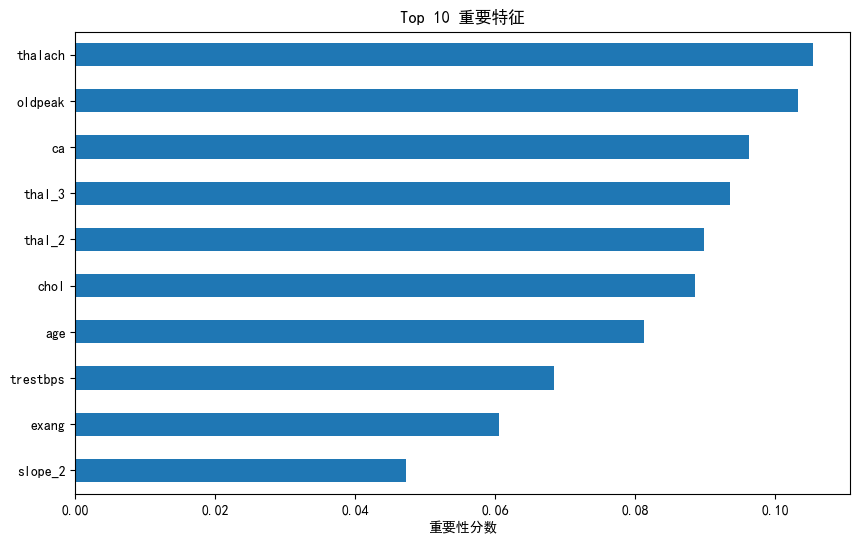


 被折叠的 条评论
为什么被折叠?
被折叠的 条评论
为什么被折叠?
 到【灌水乐园】发言


