


旋转位置编码(Rotary Position Embedding,RoPE)是一种能够将相对位置信息依赖集成Attention计算里的方法。就是在做词表映射的时候不是单一的进行一个embedding计算,还考虑位置信息。
一些资料
[1] https://arxiv.org/pdf/2104.09864
[2] https://arxiv.org/pdf/1706.03762
https://colab.research.google.com/drive/1rPk3ohrmVclqhH7uQ7qys4oznDdAhpzF
Attention
从论文里: An attention function can be described as mapping a query and a set of key-value pairs to an output. Attention即把查询向量映射成一个输出的操作。在看之前先看下embedding和qkv等几个基本概念。
Embedding
embdding的作用是词表到特征向量的映射,即把一个int的index索引映射到一个向量空间表示。比如看llama的token: https://huggingface.co/meta-llama/Llama-2-7b-hf/blob/main/tokenizer.json
截图:

vocab里面是当前模型的所有词表,比如"<unk>"对应的索引是0。通过tokenizer.endocer的编码操
作就可以将一个字段编译成一组index vector。比如:
from transformers import LlamaForCausalLM, LlamaTokenizer

tokenizer = LlamaTokenizer.from_pretrained("/model/Llama-2-7b-chat-hf")


encode = tokenizer.encode("who")
print(encode)

# [1, 1058]
# "" -> 1
# "who" -> 1058
然后得到的[1, 1058]就是embedding的输入了。embeding的计算:
>>> import torch
>>> a = torch.tensor([1])   # 输入index是1就是前面encode后的数值

>>> import torch.nn as nn
>>> embedding = nn.Embedding(3, 3)
>>> embedding.weight
Parameter containing:
tensor([[ 0.0198, -0.5562,  0.8156],
        [-0.3192, -1.2203, -0.8307],
        [-0.1649, -0.2753, -0.9075]], requires_grad=True)
>>> o = embedding(a) # 从weight里取出来对应的第1行的数值。
>>> o
tensor([[-0.3192, -1.2203, -0.8307]], grad_fn=<EmbeddingBackward0>)
embeeding的操作是根据输入的index的数值(比如这里1)然后从对应的权重(embedding.weight, 3x3)里取出对应index行索引对应的权重vector(第一行,embedding.weight[1])。即一个简单的索引操作。所以这里就有一个限制,即输入的index的大小必须要小于embedding.weight的shape(0),超出了就会挂掉。另外embedding.weight的shape(1)的大小被称为hidden size,即feature的大小。后面的linear等操作都是根据这个feature来运算的。实际上,embedding将index变成了一个高维空间的表示,可以用于模型训练推理。正常下embedding的权重第一个维度大小是vocab_size,可以查看config.json配置文件。
query、keys and values
query: 希望取查询的文本对应的查找向量,即LLM的输入经过embedding映射后的向量就是一个query vector。
keys: 和query,是对输入的文本的一个向量映射。keys里存储了所有的之前LLM推理后的context的vector数值。The key vectors are used to compute how relevant each element in the input sequence is to the query.
values: values是和query一一对应的,一个key对应一个values, These values are weighted by the attention scores (computed from the query-key interaction) to determine how much each element contributes to the final output.
也就是根据key和value,来判断当前的query和哪个key的关联性最高,分数最高。那么是怎么计算的呢?参考qkv比较清楚计算方式了。

从图中可以看到对一个query([1, 0, 2])会分别和三组key/value计算,得到三组vactor。然后再把三组vector相加得到[2, 7, 1.5],这个vector在经过重复的mlp和attention和最后的logits处理得到llm模型的输出index, 比如:

第一次输入How to predict, 经过llm根据最后的softmax后vector选取最优的输出。每个有个score. (prefill的时候全部是query,没有key value的)decode的时候,query长度都是1,然后之前的context存储在所有的key value里。
Attention is all you need
An attention function can be described as mapping a query and a set of key-value pairs to an output, where the query, keys, values, and output are all vectors. attention表示:

左图是最简单的attention操作,右边是multi head attention的图. 先看左图,输入QKV,经过计算Scaled Dot Product Attention,得到一组特征向量,然后每一组query和key/value得到一个vector(如上面qkv章节的图),然后将vector相加。计算公式 :
scaled dot product attention:

query和key的维度是。如qkv章节的图,q和k点乘,然后经过softmax之后得到一个score分数。在将这个score和V做乘法,即得到一个基于当前组k/v的输出特征向量。
一个scaled dot product的pytorch实现:
class ScaledDotProductAttention(nn.Module):
    ''' Scaled Dot-Product Attention '''

    def __init__(self, temperature, attn_dropout=0.1):
        super().__init__()
        self.temperature = temperature
        self.dropout = nn.Dropout(attn_dropout)

    def forward(self, q, k, v, mask=None):

        attn = torch.matmul(q / self.temperature, k.transpose(2, 3))

        if mask is not None:
            attn = attn.masked_fill(mask == 0, -1e9)

        attn = self.dropout(F.softmax(attn, dim=-1))
        output = torch.matmul(attn, v)

        return output, attn
Multi-Head Attention(MHA)
多头注意力机制和单个scaled dot product attention的区别是先将输入的QKV分别进行多个linear操作,然后在最后的输出vector也经过多个linear映射。这样可以将qkv的向量映射到更高维度的空间上。每个linear的输出大小可以表示为head_dim, 有多少和linear可以用head_num来表示。多头(head)即指这里head_num有几个。一般在实现的时候由于linear是线性的,所以可以将多个head合并成一个linear算子来实现,这个linear的权重大小就是head_num * head_dim(这样也自动实现了图里面的concat操作)。 一个MHA的实现:
class MultiHeadAttention(nn.Module):
    ''' Multi-Head Attention module '''

    def __init__(self, n_head, d_model, d_k, d_v, dropout=0.1):
        super().__init__()

        self.n_head = n_head
        self.d_k = d_k
        self.d_v = d_v

        self.w_qs = nn.Linear(d_model, n_head * d_k, bias=False)
        self.w_ks = nn.Linear(d_model, n_head * d_k, bias=False)
        self.w_vs = nn.Linear(d_model, n_head * d_v, bias=False)
        self.fc = nn.Linear(n_head * d_v, d_model, bias=False)

        self.attention = ScaledDotProductAttention(temperature=d_k ** 0.5)

        self.dropout = nn.Dropout(dropout)
        self.layer_norm = nn.LayerNorm(d_model, eps=1e-6)


    def forward(self, q, k, v, mask=None):

        d_k, d_v, n_head = self.d_k, self.d_v, self.n_head
        sz_b, len_q, len_k, len_v = q.size(0), q.size(1), k.size(1), v.size(1)

        residual = q

        # Pass through the pre-attention projection: b x lq x (n*dv)
        # Separate different heads: b x lq x n x dv
        q = self.w_qs(q).view(sz_b, len_q, n_head, d_k)
        k = self.w_ks(k).view(sz_b, len_k, n_head, d_k)
        v = self.w_vs(v).view(sz_b, len_v, n_head, d_v)

        # Transpose for attention dot product: b x n x lq x dv
        q, k, v = q.transpose(1, 2), k.transpose(1, 2), v.transpose(1, 2)

        if mask is not None:
            mask = mask.unsqueeze(1)   # For head axis broadcasting.

        q, attn = self.attention(q, k, v, mask=mask)

        # Transpose to move the head dimension back: b x lq x n x dv
        # Combine the last two dimensions to concatenate all the heads together: b x lq x (n*dv)
        q = q.transpose(1, 2).contiguous().view(sz_b, len_q, -1)
        q = self.dropout(self.fc(q))
        q += residual

        q = self.layer_norm(q)

        return q, attn
multi head的体现就体现在了qkv三个linear上,一般的权重大小是:
x: [bs, seq_len, hidden_size] # hidden size有embedding的输出决定
Q: [hidden_size, num_hididden_heads * head_dim] # Q有num_hiddden_heads个头,每个head大小是head dim.
K/V: [hidden_size, num_key_value_heads * head_dim] # KV的head num一样
查看每个LLM模型的head_num等参数可以看对应权重目录下的config.json
{
  "_name_or_path": "meta-llama/Llama-2-7b-hf",
  "architectures": [
    "LlamaForCausalLM"
  ],
  "bos_token_id": 1,
  "eos_token_id": 2,
  "hidden_act": "silu",
  "hidden_size": 4096,
  "initializer_range": 0.02,
  "intermediate_size": 11008,
  "max_position_embeddings": 4096,
  "model_type": "llama",
  "num_attention_heads": 32,
  "num_hidden_layers": 32,
  "num_key_value_heads": 32,
  "pretraining_tp": 1,
  "rms_norm_eps": 1e-05,
  "rope_scaling": null,
  "tie_word_embeddings": false,
  "torch_dtype": "float16",
  "transformers_version": "4.31.0.dev0",
  "use_cache": true,
  "vocab_size": 32000
}
RoPE
Positional Encoding
位置编码主要是将位置信息加入到输入vector里。啥意思,为啥呢?还是看qkv章节里的图,attention的原理是计算q和每个kv的关系向量,假设三个kv则得到三个vector,然后将三个vector做加法。这个操作就导致,如果将三组kv的顺序换掉的话还是得到一样的三个vector, 做加法后输出还是一样的, 自注意机制无法捕捉位置信息!比如输入是"I am a"和"a I am"的attention特征向量一样了,那结果肯定有问题的。所以希望在计算attention的时候除了vector之外还可以带上当前vector的位置信息。这个工作就用positionl encoding来完成。
最简单的想法是用绝对位置编码,即对每一个embedding后的vector加上一个独立的position encoding向量(比如one hot的向量,1表示位置信息,其他为0)或者根据论文里的实现通过下面方式正弦编码(Sinusoidal):
import torch
import torch.nn as nn
import numpy as np

class PositionalEncoding(nn.Module):

    def __init__(self, d_hid, n_position=5):
        super(PositionalEncoding, self).__init__()

        # Not a parameter
        self.register_buffer('pos_table', self._get_sinusoid_encoding_table(n_position, d_hid))

    def _get_sinusoid_encoding_table(self, n_position, d_hid):
        ''' Sinusoid position encoding table '''
        # TODO: make it with torch instead of numpy

        def get_position_angle_vec(position):
            return [position / np.power(10000, 2 * (hid_j // 2) / d_hid) for hid_j in range(d_hid)]

        sinusoid_table = np.array([get_position_angle_vec(pos_i) for pos_i in range(n_position)])
        sinusoid_table[:, 0::2] = np.sin(sinusoid_table[:, 0::2])  # dim 2i
        sinusoid_table[:, 1::2] = np.cos(sinusoid_table[:, 1::2])  # dim 2i+1

        return torch.FloatTensor(sinusoid_table).unsqueeze(0)

    def forward(self, x):
        return x + self.pos_table[:, :x.size(1)].clone().detach()

model = PositionalEncoding(10)
x = torch.randn([1, 10])

model(x)
输出一下sinusoid_table:
0 10 [0.0, 0.0, 0.0, 0.0, 0.0, 0.0, 0.0, 0.0, 0.0, 0.0]
1 10 [1.0, 1.0, 0.15848931924611134, 0.15848931924611134, 0.025118864315095794, 0.025118864315095794, 0.003981071705534973, 0.003981071705534973, 0.000630957344480193, 0.000630957344480193]
2 10 [2.0, 2.0, 0.3169786384922227, 0.3169786384922227, 0.05023772863019159, 0.05023772863019159, 0.007962143411069947, 0.007962143411069947, 0.001261914688960386, 0.001261914688960386]
3 10 [3.0, 3.0, 0.47546795773833406, 0.47546795773833406, 0.07535659294528739, 0.07535659294528739, 0.011943215116604919, 0.011943215116604919, 0.0018928720334405792, 0.0018928720334405792]
4 10 [4.0, 4.0, 0.6339572769844454, 0.6339572769844454, 0.10047545726038318, 0.10047545726038318, 0.015924286822139894, 0.015924286822139894, 0.002523829377920772, 0.002523829377920772]
论文里的公式:

每一行position是不一样的,然后对每个0~hidden size上,偶数位置用sin计算pe,奇数位置用cos计算pe值。这种计算的好处是不仅将position值考虑进计算,而且相邻的区域使用sin/cos进行了区分,而且由于sin/cos是有边界的函数这样也导致pe的值不会太大。
位置编码的主要目的就是将位置信息引入到embedding后的特征向量表示中,将每个kv的vector在空间表示的时候可以完全的分开。
但是相对位置编码有个问题就是和训练时候的vocab size强绑定,当推理词表长度和训练不一样,那相对位置编码就没有这么强的泛化性了。这个被称为外推性,外推性是指大模型在训练时和预测时的输入长度不一致,导致模型的泛化能力下降的问题。而且绝对位置编码还是只和当前的位置有关系,无法感知相对位置信息。
RoPE
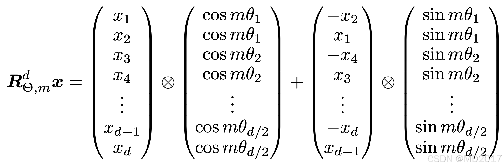
Rotary Position Embedding(RoPE)选择位置编码考虑了相对位置信息,使用旋转矩阵来实现。什么是旋转矩阵, 在计算机视觉里旋转矩阵常用来变换图像像素:

R是一个旋转矩阵,可以将像素点(x, y)进行一定的旋转变换。在rope论文里就使用了旋转矩阵来变换embedding词向量:

然后根据2维度的旋转矩阵就得到了rope层的大的旋转矩阵。从公式里看到rope的计算只和Q/K的权重有关系的,和V是没有关系的。
到这看公式有点懵了...所以对着代码先把这一部分theta的计算看懂.
transformer代码中怎么获取theta值的,即怎么到这个R?
先看Llama-2-7b-hf的参数:
{
  "_name_or_path": "meta-llama/Llama-2-7b-hf",
  "architectures": [
    "LlamaForCausalLM"
  ],
  "bos_token_id": 1,
  "eos_token_id": 2,
  "hidden_act": "silu",
  "hidden_size": 4096,
  "initializer_range": 0.02,
  "intermediate_size": 11008,
  "max_position_embeddings": 4096,
  "model_type": "llama",
  "num_attention_heads": 32,
  "num_hidden_layers": 32,
  "num_key_value_heads": 32,
  "pretraining_tp": 1,
  "rms_norm_eps": 1e-05,
  "rope_scaling": null,
  "tie_word_embeddings": false,
  "torch_dtype": "float16",
  "transformers_version": "4.31.0.dev0",
  "use_cache": true,
  "vocab_size": 32000
}
找到transfomre中对应计算的过程
从Positional Encoding的计算公式看出需要先计算一个角度theta,然后求cos/sin值。先看这一部分实现:
_compute_default_rope_parameters(https://github.com/huggingface/transformers/blob/v4.44.2/src/transformers/modeling_rope_utils.py#L29)
def _compute_default_rope_parameters(
    config: Optional[PretrainedConfig] = None,
    device: Optional["torch.device"] = None,
    seq_len: Optional[int] = None,
    **rope_kwargs,
) -> Tuple["torch.Tensor", float]:
    if config is not None and len(rope_kwargs) > 0:
        raise ValueError(
            "Unexpected arguments: `**rope_kwargs` and `config` are mutually exclusive in "
            f"`_compute_default_rope_parameters`, got `rope_kwargs`={rope_kwargs} and `config`={config}"
        )
    if len(rope_kwargs) > 0:
        base = rope_kwargs["base"]
        dim = rope_kwargs["dim"]
    elif config is not None:
        base = config.rope_theta
        partial_rotary_factor = config.partial_rotary_factor if hasattr(config, "partial_rotary_factor") else 1.0
        head_dim = getattr(config, "head_dim", config.hidden_size // config.num_attention_heads)
        dim = int(head_dim * partial_rotary_factor)

    attention_factor = 1.0  # Unused in this type of RoPE
    # head_dim:  128  dim:  128  partial_rotary_factor:  1.0
    # config.hidden_size 4096  config.num_attention_heads:  32
    # base rope theta:  10000.0

    # Compute the inverse frequencies
    inv_freq = 1.0 / (base ** (torch.arange(0, dim, 2, dtype=torch.int64).float().to(device) / dim))
    return inv_freq, attention_factor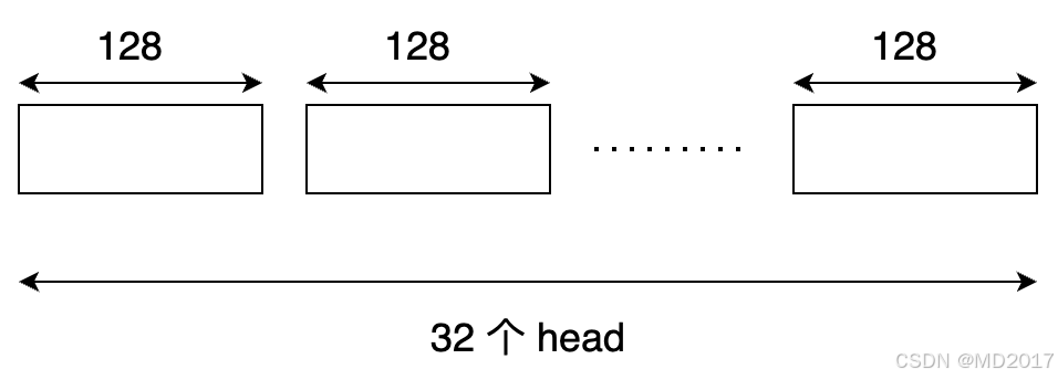
从配置里hidden_size = 4096, qkv三个的head_num = 32,所以每个head的大小就是head_dim = hidden_size / head_num = 128。这里主要的计算就一个地方:
 inv_freq = 1.0 / (base ** (torch.arange(0, dim, 2, dtype=torch.int64).float().to(device) / dim))

# 1. torch.arange(0, 128, 2)
tensor([  0,   2,   4,   6,   8,  10,  12,  14,  16,  18,  20,  22,  24,  26,
         28,  30,  32,  34,  36,  38,  40,  42,  44,  46,  48,  50,  52,  54,
         56,  58,  60,  62,  64,  66,  68,  70,  72,  74,  76,  78,  80,  82,
         84,  86,  88,  90,  92,  94,  96,  98, 100, 102, 104, 106, 108, 110,
        112, 114, 116, 118, 120, 122, 124, 126])

#2. torch.arange(0, 128, 2) / 128
tensor([0.0000, 0.0156, 0.0312, 0.0469, 0.0625, 0.0781, 0.0938, 0.1094, 0.1250,
        0.1406, 0.1562, 0.1719, 0.1875, 0.2031, 0.2188, 0.2344, 0.2500, 0.2656,
        0.2812, 0.2969, 0.3125, 0.3281, 0.3438, 0.3594, 0.3750, 0.3906, 0.4062,
        0.4219, 0.4375, 0.4531, 0.4688, 0.4844, 0.5000, 0.5156, 0.5312, 0.5469,
        0.5625, 0.5781, 0.5938, 0.6094, 0.6250, 0.6406, 0.6562, 0.6719, 0.6875,
        0.7031, 0.7188, 0.7344, 0.7500, 0.7656, 0.7812, 0.7969, 0.8125, 0.8281,
        0.8438, 0.8594, 0.8750, 0.8906, 0.9062, 0.9219, 0.9375, 0.9531, 0.9688,
        0.9844])

3. >>>  10000.0 ** (torch.arange(0, 128, 2) / 128)
tensor([1.0000e+00, 1.1548e+00, 1.3335e+00, 1.5399e+00, 1.7783e+00, 2.0535e+00,
        2.3714e+00, 2.7384e+00, 3.1623e+00, 3.6517e+00, 4.2170e+00, 4.8697e+00,
        5.6234e+00, 6.4938e+00, 7.4989e+00, 8.6596e+00, 1.0000e+01, 1.1548e+01,
        1.3335e+01, 1.5399e+01, 1.7783e+01, 2.0535e+01, 2.3714e+01, 2.7384e+01,
        3.1623e+01, 3.6517e+01, 4.2170e+01, 4.8697e+01, 5.6234e+01, 6.4938e+01,
        7.4989e+01, 8.6596e+01, 1.0000e+02, 1.1548e+02, 1.3335e+02, 1.5399e+02,
        1.7783e+02, 2.0535e+02, 2.3714e+02, 2.7384e+02, 3.1623e+02, 3.6517e+02,
        4.2170e+02, 4.8697e+02, 5.6234e+02, 6.4938e+02, 7.4989e+02, 8.6596e+02,
        1.0000e+03, 1.1548e+03, 1.3335e+03, 1.5399e+03, 1.7783e+03, 2.0535e+03,
        2.3714e+03, 2.7384e+03, 3.1623e+03, 3.6517e+03, 4.2170e+03, 4.8697e+03,
        5.6234e+03, 6.4938e+03, 7.4989e+03, 8.6596e+03])

4. inv_freq = 1.0 / (10000.0 ** (torch.arange(0, 128, 2) / 128))
tensor([1.0000e+00, 8.6596e-01, 7.4989e-01, 6.4938e-01, 5.6234e-01, 4.8697e-01,
        4.2170e-01, 3.6517e-01, 3.1623e-01, 2.7384e-01, 2.3714e-01, 2.0535e-01,
        1.7783e-01, 1.5399e-01, 1.3335e-01, 1.1548e-01, 1.0000e-01, 8.6596e-02,
        7.4989e-02, 6.4938e-02, 5.6234e-02, 4.8697e-02, 4.2170e-02, 3.6517e-02,
        3.1623e-02, 2.7384e-02, 2.3714e-02, 2.0535e-02, 1.7783e-02, 1.5399e-02,
        1.3335e-02, 1.1548e-02, 1.0000e-02, 8.6596e-03, 7.4989e-03, 6.4938e-03,
        5.6234e-03, 4.8697e-03, 4.2170e-03, 3.6517e-03, 3.1623e-03, 2.7384e-03,
        2.3714e-03, 2.0535e-03, 1.7783e-03, 1.5399e-03, 1.3335e-03, 1.1548e-03,
        1.0000e-03, 8.6596e-04, 7.4989e-04, 6.4938e-04, 5.6234e-04, 4.8697e-04,
        4.2170e-04, 3.6517e-04, 3.1623e-04, 2.7384e-04, 2.3714e-04, 2.0535e-04,
        1.7783e-04, 1.5399e-04, 1.3335e-04, 1.1548e-04])
上面的计算其实就对应到下面的公式:

这里d = 128,即计算出了所有的theta数值。以2为间隔,输出的inv_freq大小是[64]
计算llama attention
得到了所有的theta值后怎么在attention里计算呢?transformers/src/transformers/models/llama/modeling_llama.py at v4.44.2 · huggingface/transformers · GitHub
先乘上position的信息:
freqs = (inv_freq_expanded.float() @ position_ids_expanded.float()).transpose(1, 2)这里position_ids_expanded是位置信息,比如第一个token的position_ids = [0], 第二个是[1],依次类推。如果文本长度设置的是10,那么这个position_ids = [0, 1, 2, 3, 4, 5, 6, 7,8, 9]。 乘法之后freqs为:
freq:
 tensor([[[0.0000e+00, 0.0000e+00, 0.0000e+00, 0.0000e+00, 0.0000e+00,
          0.0000e+00, 0.0000e+00, 0.0000e+00, 0.0000e+00, 0.0000e+00,
          0.0000e+00, 0.0000e+00, 0.0000e+00, 0.0000e+00, 0.0000e+00,
          0.0000e+00, 0.0000e+00, 0.0000e+00, 0.0000e+00, 0.0000e+00,
          0.0000e+00, 0.0000e+00, 0.0000e+00, 0.0000e+00, 0.0000e+00,
          0.0000e+00, 0.0000e+00, 0.0000e+00, 0.0000e+00, 0.0000e+00,
          0.0000e+00, 0.0000e+00, 0.0000e+00, 0.0000e+00, 0.0000e+00,
          0.0000e+00, 0.0000e+00, 0.0000e+00, 0.0000e+00, 0.0000e+00,
          0.0000e+00, 0.0000e+00, 0.0000e+00, 0.0000e+00, 0.0000e+00,
          0.0000e+00, 0.0000e+00, 0.0000e+00, 0.0000e+00, 0.0000e+00,
          0.0000e+00, 0.0000e+00, 0.0000e+00, 0.0000e+00, 0.0000e+00,
          0.0000e+00, 0.0000e+00, 0.0000e+00, 0.0000e+00, 0.0000e+00,
          0.0000e+00, 0.0000e+00, 0.0000e+00, 0.0000e+00],
         [1.0000e+00, 8.6596e-01, 7.4989e-01, 6.4938e-01, 5.6234e-01,
          4.8697e-01, 4.2170e-01, 3.6517e-01, 3.1623e-01, 2.7384e-01,
          2.3714e-01, 2.0535e-01, 1.7783e-01, 1.5399e-01, 1.3335e-01,
          1.1548e-01, 1.0000e-01, 8.6596e-02, 7.4989e-02, 6.4938e-02,
          5.6234e-02, 4.8697e-02, 4.2170e-02, 3.6517e-02, 3.1623e-02,
          2.7384e-02, 2.3714e-02, 2.0535e-02, 1.7783e-02, 1.5399e-02,
          1.3335e-02, 1.1548e-02, 1.0000e-02, 8.6596e-03, 7.4989e-03,
          6.4938e-03, 5.6234e-03, 4.8697e-03, 4.2170e-03, 3.6517e-03,
          3.1623e-03, 2.7384e-03, 2.3714e-03, 2.0535e-03, 1.7783e-03,
          1.5399e-03, 1.3335e-03, 1.1548e-03, 1.0000e-03, 8.6596e-04,
          7.4989e-04, 6.4938e-04, 5.6234e-04, 4.8697e-04, 4.2170e-04,
          3.6517e-04, 3.1623e-04, 2.7384e-04, 2.3714e-04, 2.0535e-04,
          1.7783e-04, 1.5399e-04, 1.3335e-04, 1.1548e-04]]])
tensor([[[2.0000e+00, 1.7319e+00, 1.4998e+00, 1.2988e+00, 1.1247e+00,
          9.7394e-01, 8.4339e-01, 7.3035e-01, 6.3246e-01, 5.4768e-01,
          4.7427e-01, 4.1071e-01, 3.5566e-01, 3.0799e-01, 2.6670e-01,
          2.3096e-01, 2.0000e-01, 1.7319e-01, 1.4998e-01, 1.2988e-01,
          1.1247e-01, 9.7394e-02, 8.4339e-02, 7.3035e-02, 6.3246e-02,
          5.4768e-02, 4.7427e-02, 4.1071e-02, 3.5566e-02, 3.0799e-02,
          2.6670e-02, 2.3096e-02, 2.0000e-02, 1.7319e-02, 1.4998e-02,
          1.2988e-02, 1.1247e-02, 9.7394e-03, 8.4339e-03, 7.3035e-03,
          6.3246e-03, 5.4768e-03, 4.7427e-03, 4.1071e-03, 3.5566e-03,
          3.0799e-03, 2.6670e-03, 2.3096e-03, 2.0000e-03, 1.7319e-03,
          1.4998e-03, 1.2988e-03, 1.1247e-03, 9.7394e-04, 8.4339e-04,
          7.3035e-04, 6.3246e-04, 5.4768e-04, 4.7427e-04, 4.1070e-04,
          3.5566e-04, 3.0799e-04, 2.6670e-04, 2.3096e-04]]])
....
位置为0的时候freq都是0, 1的时候是inv_freq, 2的时候就是freq=2*inv_freq,依次类推。
下面计算sin/cos
emb = torch.cat((freqs, freqs), dim=-1)
# emb先把两个freqs拼接一起,得到一个128维度的输出。
# 当position = 1, emb
         [1.0000e+00, 8.6596e-01, 7.4989e-01, 6.4938e-01, 5.6234e-01,
          4.8697e-01, 4.2170e-01, 3.6517e-01, 3.1623e-01, 2.7384e-01,
          2.3714e-01, 2.0535e-01, 1.7783e-01, 1.5399e-01, 1.3335e-01,
          1.1548e-01, 1.0000e-01, 8.6596e-02, 7.4989e-02, 6.4938e-02,
          5.6234e-02, 4.8697e-02, 4.2170e-02, 3.6517e-02, 3.1623e-02,
          2.7384e-02, 2.3714e-02, 2.0535e-02, 1.7783e-02, 1.5399e-02,
          1.3335e-02, 1.1548e-02, 1.0000e-02, 8.6596e-03, 7.4989e-03,
          6.4938e-03, 5.6234e-03, 4.8697e-03, 4.2170e-03, 3.6517e-03,
          3.1623e-03, 2.7384e-03, 2.3714e-03, 2.0535e-03, 1.7783e-03,
          1.5399e-03, 1.3335e-03, 1.1548e-03, 1.0000e-03, 8.6596e-04,
          7.4989e-04, 6.4938e-04, 5.6234e-04, 4.8697e-04, 4.2170e-04,
          3.6517e-04, 3.1623e-04, 2.7384e-04, 2.3714e-04, 2.0535e-04,
          1.7783e-04, 1.5399e-04, 1.3335e-04, 1.1548e-04, 1.0000e+00,
          8.6596e-01, 7.4989e-01, 6.4938e-01, 5.6234e-01, 4.8697e-01,
          4.2170e-01, 3.6517e-01, 3.1623e-01, 2.7384e-01, 2.3714e-01,
          2.0535e-01, 1.7783e-01, 1.5399e-01, 1.3335e-01, 1.1548e-01,
          1.0000e-01, 8.6596e-02, 7.4989e-02, 6.4938e-02, 5.6234e-02,
          4.8697e-02, 4.2170e-02, 3.6517e-02, 3.1623e-02, 2.7384e-02,
          2.3714e-02, 2.0535e-02, 1.7783e-02, 1.5399e-02, 1.3335e-02,
          1.1548e-02, 1.0000e-02, 8.6596e-03, 7.4989e-03, 6.4938e-03,
          5.6234e-03, 4.8697e-03, 4.2170e-03, 3.6517e-03, 3.1623e-03,
          2.7384e-03, 2.3714e-03, 2.0535e-03, 1.7783e-03, 1.5399e-03,
          1.3335e-03, 1.1548e-03, 1.0000e-03, 8.6596e-04, 7.4989e-04,
          6.4938e-04, 5.6234e-04, 4.8697e-04, 4.2170e-04, 3.6517e-04,
          3.1623e-04, 2.7384e-04, 2.3714e-04, 2.0535e-04, 1.7783e-04,
          1.5399e-04, 1.3335e-04, 1.1548e-04]]])


cos = emb.cos()
sin = emb.sin()
# position = 1时输出:
# cos: [0.5403, 0.6479, 0.7318, 0.7965, 0.8460, 0.8838, 0.9124, 0.9341,
          0.9504, 0.9627, 0.9720, 0.9790, 0.9842, 0.9882, 0.9911, 0.9933,
          0.9950, 0.9963, 0.9972, 0.9979, 0.9984, 0.9988, 0.9991, 0.9993,
          0.9995, 0.9996, 0.9997, 0.9998, 0.9998, 0.9999, 0.9999, 0.9999,
          0.9999, 1.0000, 1.0000, 1.0000, 1.0000, 1.0000, 1.0000, 1.0000,
          1.0000, 1.0000, 1.0000, 1.0000, 1.0000, 1.0000, 1.0000, 1.0000,
          1.0000, 1.0000, 1.0000, 1.0000, 1.0000, 1.0000, 1.0000, 1.0000,
          1.0000, 1.0000, 1.0000, 1.0000, 1.0000, 1.0000, 1.0000, 1.0000,
          0.5403, 0.6479, 0.7318, 0.7965, 0.8460, 0.8838, 0.9124, 0.9341,
          0.9504, 0.9627, 0.9720, 0.9790, 0.9842, 0.9882, 0.9911, 0.9933,
          0.9950, 0.9963, 0.9972, 0.9979, 0.9984, 0.9988, 0.9991, 0.9993,
          0.9995, 0.9996, 0.9997, 0.9998, 0.9998, 0.9999, 0.9999, 0.9999,
          0.9999, 1.0000, 1.0000, 1.0000, 1.0000, 1.0000, 1.0000, 1.0000,
          1.0000, 1.0000, 1.0000, 1.0000, 1.0000, 1.0000, 1.0000, 1.0000,
          1.0000, 1.0000, 1.0000, 1.0000, 1.0000, 1.0000, 1.0000, 1.0000,
          1.0000, 1.0000, 1.0000, 1.0000, 1.0000, 1.0000, 1.0000, 1.0000]]]

# sin:
         [8.4147e-01, 7.6172e-01, 6.8156e-01, 6.0469e-01, 5.3317e-01,
          4.6795e-01, 4.0931e-01, 3.5711e-01, 3.1098e-01, 2.7043e-01,
          2.3492e-01, 2.0391e-01, 1.7689e-01, 1.5338e-01, 1.3296e-01,
          1.1522e-01, 9.9833e-02, 8.6488e-02, 7.4919e-02, 6.4893e-02,
          5.6204e-02, 4.8678e-02, 4.2157e-02, 3.6509e-02, 3.1618e-02,
          2.7381e-02, 2.3712e-02, 2.0534e-02, 1.7782e-02, 1.5399e-02,
          1.3335e-02, 1.1548e-02, 9.9998e-03, 8.6595e-03, 7.4989e-03,
          6.4938e-03, 5.6234e-03, 4.8697e-03, 4.2170e-03, 3.6517e-03,
          3.1623e-03, 2.7384e-03, 2.3714e-03, 2.0535e-03, 1.7783e-03,
          1.5399e-03, 1.3335e-03, 1.1548e-03, 1.0000e-03, 8.6596e-04,
          7.4989e-04, 6.4938e-04, 5.6234e-04, 4.8697e-04, 4.2170e-04,
          3.6517e-04, 3.1623e-04, 2.7384e-04, 2.3714e-04, 2.0535e-04,
          1.7783e-04, 1.5399e-04, 1.3335e-04, 1.1548e-04, 8.4147e-01,
          7.6172e-01, 6.8156e-01, 6.0469e-01, 5.3317e-01, 4.6795e-01,
          4.0931e-01, 3.5711e-01, 3.1098e-01, 2.7043e-01, 2.3492e-01,
          2.0391e-01, 1.7689e-01, 1.5338e-01, 1.3296e-01, 1.1522e-01,
          9.9833e-02, 8.6488e-02, 7.4919e-02, 6.4893e-02, 5.6204e-02,
          4.8678e-02, 4.2157e-02, 3.6509e-02, 3.1618e-02, 2.7381e-02,
          2.3712e-02, 2.0534e-02, 1.7782e-02, 1.5399e-02, 1.3335e-02,
          1.1548e-02, 9.9998e-03, 8.6595e-03, 7.4989e-03, 6.4938e-03,
          5.6234e-03, 4.8697e-03, 4.2170e-03, 3.6517e-03, 3.1623e-03,
          2.7384e-03, 2.3714e-03, 2.0535e-03, 1.7783e-03, 1.5399e-03,
          1.3335e-03, 1.1548e-03, 1.0000e-03, 8.6596e-04, 7.4989e-04,
          6.4938e-04, 5.6234e-04, 4.8697e-04, 4.2170e-04, 3.6517e-04,
          3.1623e-04, 2.7384e-04, 2.3714e-04, 2.0535e-04, 1.7783e-04,
          1.5399e-04, 1.3335e-04, 1.1548e-04]]])

cos = cos * self.attention_scaling # scaling一般是1
sin = sin * self.attention_scaling
这里为啥有一个将两个freq拼接成128的tensor的操作呢,主要是为了方便后面cos/sin计算,后面讲。这俩的theta是完全一样的。结合论文里最重要的一张图就可以理解了:
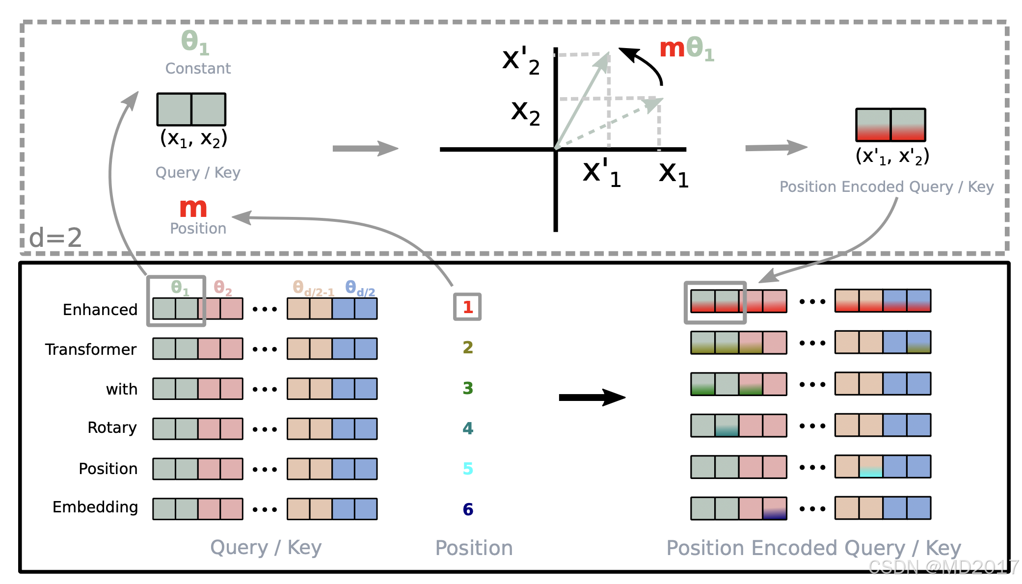
这里d=128, 在position=1的时候我们通过上面的计算得到一个64维度的theta,然后对qk分别进行变换,通过上面的图可以看到原始的qk向量x1,x2经过theta变换之后得到x1', x2'(position encoded query/key)。
这里旋转矩阵是怎么对qk计算的呢?看代码:
query_states, key_states = apply_rotary_pos_emb(query_states, key_states, cos, sin)
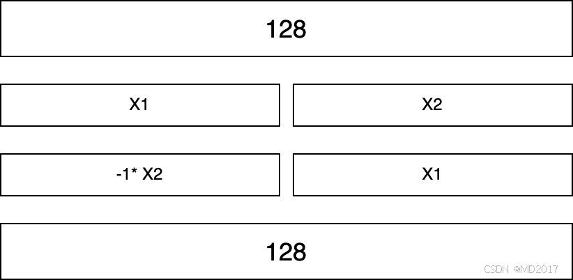
def rotate_half(x):
"""Rotates half the hidden dims of the input."""
x1 = x[..., : x.shape[-1] // 2]
x2 = x[..., x.shape[-1] // 2 :]
o = torch.cat((-x2, x1), dim=-1)
return o
def apply_rotary_pos_emb(q, k, cos, sin, position_ids=None, unsqueeze_dim=1):
"""Applies Rotary Position Embedding to the query and key tensors.
Args:
q (`torch.Tensor`): The query tensor.
k (`torch.Tensor`): The key tensor.
cos (`torch.Tensor`): The cosine part of the rotary embedding.
sin (`torch.Tensor`): The sine part of the rotary embedding.
position_ids (`torch.Tensor`, *optional*):
Deprecated and unused.
unsqueeze_dim (`int`, *optional*, defaults to 1):
The 'unsqueeze_dim' argument specifies the dimension along which to unsqueeze cos[position_ids] and
sin[position_ids] so that they can be properly broadcasted to the dimensions of q and k. For example, note
that cos[position_ids] and sin[position_ids] have the shape [batch_size, seq_len, head_dim]. Then, if q and
k have the shape [batch_size, heads, seq_len, head_dim], then setting unsqueeze_dim=1 makes
cos[position_ids] and sin[position_ids] broadcastable to the shapes of q and k. Similarly, if q and k have
the shape [batch_size, seq_len, heads, head_dim], then set unsqueeze_dim=2.
Returns:
`tuple(torch.Tensor)` comprising of the query and key tensors rotated using the Rotary Position Embedding.
"""
cos = cos.unsqueeze(unsqueeze_dim)
sin = sin.unsqueeze(unsqueeze_dim)
q_embed = (q * cos) + (rotate_half(q) * sin)
k_embed = (k * cos) + (rotate_half(k) * sin)
return q_embed, k_embed
apply_rotary_pos_emb函数输入是qkstate和cos,sin值,qk的大小:
query_states = self.q_proj(hidden_states)
key_states = self.k_proj(hidden_states)
value_states = self.v_proj(hidden_states)

query_states = query_states.view(bsz, q_len, self.num_heads, self.head_dim).transpose(1, 2)
key_states = key_states.view(bsz, q_len, self.num_key_value_heads, self.head_dim).transpose(1, 2)
value_states = value_states.view(bsz, q_len, self.num_key_value_heads, self.head_dim).transpose(1, 2)
qkv都是经过三个proj linear层后的特征向量,这里以q为例子, seq_len=10的话。大小是[1, 10, 32, 128]. 但是这里做了一个transpose(1, 2),输出就是[1, 32, 10, 128]
然后对这个q计算rotate_half,即把后面一半的数取出来*-1放到前面:
然后计算q_embed = (q * cos) + (rotate_half(q) * sin),这里是实现下面的公式:
这个步骤实现的是将cos/sin作用于qk向量中。
但是这里有个小疑问,根据rotate_haf的方式画了一下计算逻辑:
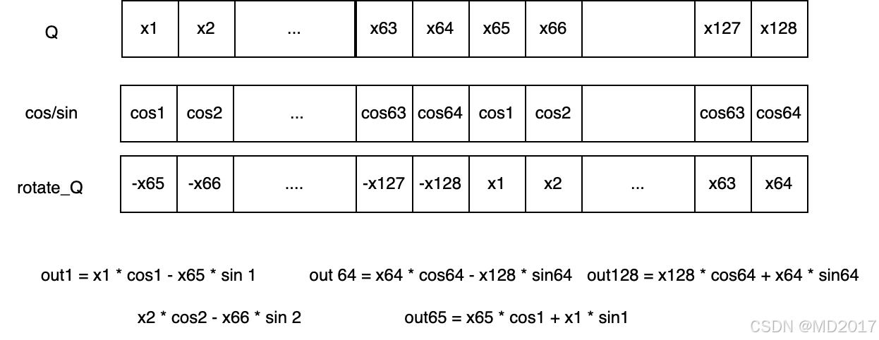
q1 = x1 * cos1 - x65 * sin1.但是按照公式应该是 x1 * cos1 - x2 * sin2。rotate_q算错了?后面看吧。


 被折叠的 条评论
为什么被折叠?
被折叠的 条评论
为什么被折叠?
 到【灌水乐园】发言


