对抗训练-smart 论文阅读笔记

对抗训练-smart 论文阅读笔记

SMART: Robust and Efficient Fine-Tuning for Pre-trained NaturalLanguage Models through Principled Regularized Optimization

---

• 论文地址 :https://arxiv.org/abs/1911.03437
• code地址 : Fine-tuning code and models
• 时间 : 2020-10
• 机构 : microsoft,gatech
• 关键词: 对抗训练 NLP BERT
• 效果评估:（2020-10） pro-posed framework achieves new state-of-the-artperformance on a number of NLP tasks includ-ing GLUE, SNLI, SciTail and ANLI. More-over, it also outperforms the state-of-the-art T5model, which is the largest pre-trained modelcontaining 11 billion parameters, on GLUE

---

简介

文中作者提出了一个新的框架SMART，用于对预先训练好的语言模型进行微调时 增加其鲁棒性，关键点有两处：

1. Smoothness-Inducing Adversarial Regularization
2. Bregman Proximal Point Optimization

Smoothness-Inducing Adversarial Regularization

模型: $f(\cdot ;\theta )$
数据个数: $n$
数据: { ( x i , y i ) } i = 1 n \{(x_i,y_i)\}_{i=1}^n {(xi​,yi​)}i=1n​
\qquad $x_i$表示输入语句的embedding，可以从模型的第一个embedding层获取到。
\qquad $y_i$表示对应的label
文中主要是在fine-tuning时优化的下面的函数:
$$mi{n}_{\theta }\mathcal{F}(\theta )=\mathcal{L}(\theta )+{\lambda }_s\mathcal{R}(\theta )\text{\hspace{1em}(1)}$$
这里：
\qquad $\mathcal{L}(\theta )$ 是整体的loss：$\mathcal{L}=\frac{1}{n}{\sum }_{i=1}^{n}l(f(x_i;\theta ),y_i)$,$其中l(\cdot ,\cdot )$ 是损失函数由具体的任务决定；
\qquad ${\lambda }_s>0$是一个可调的参数；
${\mathcal{R}}_s(\theta )$就是 smoothness-inducing adversarial regularizer，具体如下:
$$\mathcal{R}(\theta )=\frac{1}{n}\sum _{i=1}^{n}ma{x}_{\Vert \widetilde{x_i}-x_i{\Vert }_p\le ϵ}{l}_s(f(\widetilde{x_i};\theta ),f(x_i;\theta ))$$
\qquad\qquad 其中$ϵ>0$是一个可调的参数，比如在一个分类任务中模型$f(\cdot ;\theta )$输出概率分布，$l_s$可以选择为对称KL-散度如：
$$l_s(P,Q)={\mathcal{D}}_{KL}(P\Vert Q)+{\mathcal{D}}_{KL}(Q\Vert P)$$
\qquad\qquad 在一个回归任务中，模型$f(\cdot ;\theta )$输出一个值，$l_s$可以选择为方差损失如:$l_s(p,q)=(p-q{)}^2$.这样就将$\mathcal{R}(\theta )$的计算转为一个求最大值的问题，并且通过映射到梯度上升中被有效解决。

作者又介绍了这个smoothness-inducing adversarial regularizer 本质是用来衡量$f$在度量函数$l_s$下的局部利普希茨连续条件性，更谨慎的说是当我们给一个小的干扰（$l_p$ 范数小于$ϵ$）到$x_i$时，$f$的输出不会有太大变化。简而言之：smoothness-inducing adversarial regularizer $就是在一定扰动范围内要求模型输出尽可能一致的概率分{布}^{[2]}$ 因此通过对公式（1）求最小值来达到 使$f$对于 所有$x_i$的领域输出更平滑，这样一个平滑引导对解决数据量比较缺乏的的目标任务的过拟合问题与提升泛化能力有特别的帮助。如下面插图所示:

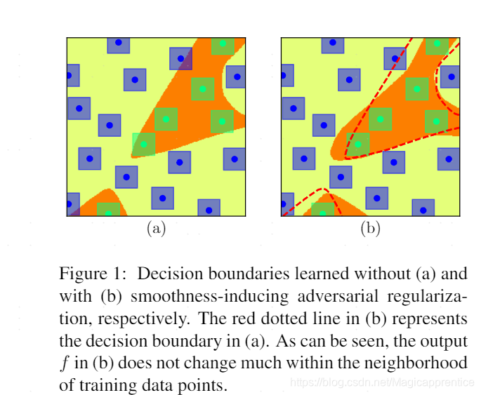
图1: (a)（b）分别是没有使用smoothness-indusing adversarial regularization 和使用 学习到的决策边界，b图中红色的虚线表示a中的决策边界，正如我们所看到的，b中$f$的输出在训练数据点的周围输出并没有太大改变。

\qquad 作者指出衡量局部的lipschitz连续性的想法类似于可以追溯到1960年代的有关稳健统计文献中的局部偏移敏感度准则。这个准则被用于衡量一个估计值对样本点中某一个值的依赖性。

Bregman Proximal Point Optimization

作者提出了一个类似于Bregman 近似点优化的方法来解决公式（1），这个优化方法采用对每次迭代都施加较大的惩罚。具体来说，我们使用一个预训练的模型作为初始化，用$f(\cdot ;{\theta }_0)$表示，在第$(t+1)$ 次迭代，$vanillaBregmanproximalpoint(VBPP)$ 方法使用:
$${\theta }_{t+1}=argmi{n}_{\theta }\mathcal{F}(\theta )+\mu {\mathcal{D}}_{Breg}(\theta ,{\theta }_t),\text{\hspace{1em}(2)}$$

这里$\mu >0$是一个可调的参数，${\mathcal{D}}_{Breg}(\cdot ,\cdot )$ 是Bregman divergence${}^{[4]}$（布雷格曼散度）,定义如下:
$${\mathcal{D}}_{Breg}(\theta ,{\theta }_t)=\frac{1}{n}\sum _{i=1}^n{l}_s(f(x_i;\theta ),f(x_i;{\theta }_t)),$$
$l_s$已在上节定义，可以看出当$\mu$比较大的时候，在VBPP 方法的每一轮迭代时， 布雷格曼散度本质上是一个强大的正则化器，可以防止${\theta }_{t+1}$ 与之前迭代的${\theta }_t$相差太大。这种方法在现有的优化相关的文献中被称为信任区域类型的迭代。因此Bregman近似点法可以有效的保留预训练模型中的使用的预训练数据里的知识。由于对于VBPP每个子问题(2) 并不允许一个封闭式的解决方案，因此需要使用类似于随机梯度下降类型的算法解决如(adam).作者指出不需要每一步都解决每个子问题，除非到最后收敛时。少量的迭代足以输出可靠的初始解决方案来解决下一个子问题。（这句话不太明白）
此外，布雷格曼近似点方法能够适应机器学习模型的信息几何学，并且与标准近似点方法(如${\mathcal{D}}_{Breg}(\theta ,{\theta }_t)=\Vert \theta -{\theta }_t{\Vert }_2^2$)相比在很多应用场景下具有更好的计算性能。

Acceleration by Momentum（动量加速）

与现有的文献中的其他优化方法类似，作者也通过加入额外的动量到更新过程中来加速Bregman 近点方法。具体来说，在第$(t+1)$此迭代中，动量布雷格曼近似点（MBPP） 使用:
$${\theta }_{t+1}=argmi{n}_{\theta }\mathcal{F}(\theta )+\mu {\mathcal{D}}_{Breg}(\theta ,\widetilde{{\theta }_t}),\text{\hspace{1em}(3)}$$
这里$\widetilde{{\theta }_t}=(1-\beta ){\theta }_t+\beta \widetilde{{\theta }_{t-1}}$ 是指数移动平均，$\beta \in (0,1)$ 是动量参数。MBPP方法在已知的文献中也被称为“Mean Teacher” 方法，并且也在一些流行的半监督学习的基准上取得了sota的效果。 为方便起见，作者总结MBPP方法为如下的$Algorithm-1$:

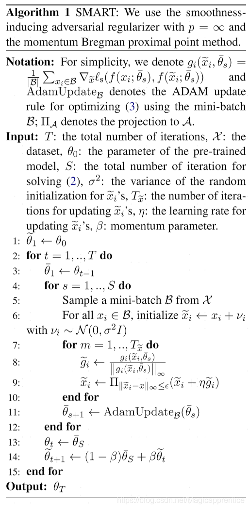
翻译一下

算法SMART：我们使用$p=\infty$,smoothness-inducing adversarial regularizer(光滑诱导对抗正则化) 和 动量布雷格曼近似点法。
符号定义: 为了简单起见，$g_i(\widetilde{x_i},\overline{{\theta }_s})=\frac{1}{\mathcal{B}}{\sum }_{x_i\in \mathcal{B}}{\nabla }_{\tilde{x}}{l}_s(f(x_i;{\bar{\theta }}_s),f({\tilde{x}}_i;{\bar{\theta }}_s))$ ；$AdamUpdat{e}_{\mathcal{B}}$ 表示ADAM 使用batchsize为$\mathcal{B}$，在公式（3）的优化上的更新规则；${\prod }_{\mathcal{A}}$ 表示投影到 $\mathcal{A}$
输入: $T$ : 总共的迭代的次数，$\mathcal{X}$:数据集，${\theta }_0$:预训练模型的参数，$S$:解决公式(2)需要的迭代步数，${\sigma }^2$:表示${\tilde{x}}_i$随机初始化的方差，$T_{\tilde{x}}$：表示更新${\tilde{x}}_i$迭代的次数，$\eta$:表示更新${\tilde{x}}_i$的学习率，$\beta$:表示动量参数。
$\tilde\theta_i \leftarrow \theta_0 $
for $t=1,..,T$ do
${\bar{\theta }}_i\leftarrow {\theta }_{t-1}$
\qquad for $s=1,..,S$ do
\qquad \qquad 从数据集$\mathcal{X}$中取mini-batch$\mathcal{B}$个样本
\qquad \qquad 对于所有的$x_i\in \mathcal{B}$,初始化增加扰动后的${\tilde{x}}_i\leftarrow x_i+v_i,v_i\sim \mathcal{N}(0,{\sigma }^{2}I)$
\qquad\qquad for $m=1,..,T_{\tilde{x}}$ do
$g_i\leftarrow \frac{g_i(\widetilde{x_i},\overline{{\theta }_s})}{\Vert g_i(\widetilde{x_i},\overline{{\theta }_s}){\Vert }_{\infty }}$
${\tilde{x}}_i\leftarrow {\prod }_{\Vert {\tilde{x}}_i-x{\Vert }_{\infty }}\le ϵ({\tilde{x}}_i+\eta {\tilde{g}}_i)$
\qquad\qquad end for
${\bar{\theta }}_s+1\leftarrow AdamUpdat{e}_{\mathcal{B}}({\bar{\theta }}_s)$
${\theta }_t\leftarrow {\bar{\theta }}_S$
${\theta }_{t+1}\leftarrow (1-\beta ){\bar{\theta }}_S+\beta {\tilde{\theta }}_t$

end for
$\delta$

后面是实验时使用的各种参数与配置，就不再描述了，下面结合下源码分析下作者是如何实现上面两个步骤的。

总结

文中通过两种方法来提高微调的结果：
1、训练过程中加入对embded的随机扰动，要求模型输出尽可能与扰动前一致的概率分布。
2、在模型参数更新时，修改Adam的结果，要求尽可能参数与预训练时的参数分布相近。尽可能少改变。。

源码分析

作者源代码如下:
https://github.com/namisan/mt-dnn/blob/471f717a25ab744e710591274c3ec098f5f4d0ad/mt_dnn/perturbation.py

from copy import deepcopy
import torch
import logging
import random
from torch.nn import Parameter
from functools import wraps
import torch.nn.functional as F
from data_utils.task_def import TaskType
from data_utils.task_def import EncoderModelType
from .loss import stable_kl 

logger = logging.getLogger(__name__)

def generate_noise(embed, mask, epsilon=1e-5):
	#生成与embed 同尺寸方差为epsion的符合正态分布的noise
    noise = embed.data.new(embed.size()).normal_(0, 1) *  epsilon
    noise.detach()
    noise.requires_grad_()
    return noise


class SmartPerturbation():
    def __init__(self,
                 epsilon=1e-6,
                 multi_gpu_on=False,
                 step_size=1e-3,
                 noise_var=1e-5,
                 norm_p='inf',
                 k=1,
                 fp16=False,
                 encoder_type=EncoderModelType.BERT,
                 loss_map=[],
                 norm_level=0):
        super(SmartPerturbation, self).__init__()
        self.epsilon = epsilon 
        # eta 更新扰动后的x_i的学习率
        self.step_size = step_size
        self.multi_gpu_on = multi_gpu_on
        self.fp16 = fp16
        self.K = k
        # sigma 生成扰动噪音的方差
        self.noise_var = noise_var 
        self.norm_p = norm_p
        self.encoder_type = encoder_type 
        self.loss_map = loss_map 
        self.norm_level = norm_level > 0
        assert len(loss_map) > 0


    def _norm_grad(self, grad, eff_grad=None, sentence_level=False):
    	# 计算梯度 以及 有效梯度的 方向
        if self.norm_p == 'l2':
            if sentence_level:
                direction = grad / (torch.norm(grad, dim=(-2, -1), keepdim=True) + self.epsilon)
            else:
                direction = grad / (torch.norm(grad, dim=-1, keepdim=True) + self.epsilon)
        elif self.norm_p == 'l1':
            direction = grad.sign()
        else:
            if sentence_level:
                direction = grad / (grad.abs().max((-2, -1), keepdim=True)[0] + self.epsilon)
            else:
                direction = grad / (grad.abs().max(-1, keepdim=True)[0] + self.epsilon)
                eff_direction = eff_grad / (grad.abs().max(-1, keepdim=True)[0] + self.epsilon)
        return direction, eff_direction

    def forward(self, model,
                logits,
                input_ids,
                token_type_ids,
                attention_mask,
                premise_mask=None,
                hyp_mask=None,
                task_id=0,
                task_type=TaskType.Classification,
                pairwise=1):
        # adv training
        assert task_type in set([TaskType.Classification, TaskType.Ranking, TaskType.Regression]), 'Donot support {} yet'.format(task_type)
        vat_args = [input_ids, token_type_ids, attention_mask, premise_mask, hyp_mask, task_id, 1] 

        # init delta
        # 输出 embded 
        embed = model(*vat_args)
        noise = generate_noise(embed, attention_mask, epsilon=self.noise_var)
        for step in range(0, self.K):
            vat_args = [input_ids, token_type_ids, attention_mask, premise_mask, hyp_mask, task_id, 2, embed + noise]
            # 使用加入噪音的embed 输出预测结果
            adv_logits = model(*vat_args)
            if task_type == TaskType.Regression:
            	# 回归问题使用 mse loss 评估与原始embedded输出的差异
                adv_loss = F.mse_loss(adv_logits, logits.detach(), reduction='sum')
            else:
                if task_type == TaskType.Ranking:
                    adv_logits = adv_logits.view(-1, pairwise)
                # 排序或者分类使用kl散度衡量两者之间的差异
                adv_loss = stable_kl(adv_logits, logits.detach(), reduce=False) 
            #  分布损失与 扰动之间的梯度
            delta_grad, = torch.autograd.grad(adv_loss, noise, only_inputs=True, retain_graph=False)
            # 梯度的范数
            norm = delta_grad.norm()
            if (torch.isnan(norm) or torch.isinf(norm)):
                return 0
            # 更新到主要训练过程中的梯度 为扰动与原始输出差异损失对扰动求出的梯度 乘以 扰动的学习率
            eff_delta_grad = delta_grad * self.step_size
            # 
            delta_grad = noise + delta_grad * self.step_size
            noise, eff_noise = self._norm_grad(delta_grad, eff_grad=eff_delta_grad, sentence_level=self.norm_level)
            noise = noise.detach()
            noise.requires_grad_()
        vat_args = [input_ids, token_type_ids, attention_mask, premise_mask, hyp_mask, task_id, 2, embed + noise]
        adv_logits = model(*vat_args)
        if task_type == TaskType.Ranking:
            adv_logits = adv_logits.view(-1, pairwise)
        adv_lc = self.loss_map[task_id]
        adv_loss = adv_lc(logits, adv_logits, ignore_index=-1)
        return adv_loss, embed.detach().abs().mean(), eff_noise.detach().abs().mean()

---

（备注） 暂时没有看到作者源码中有关于bregman divergence 与optimizer相结合的源码实现。

参考文献

[1]SMART: Robust and Efficient Fine-Tuning for Pre-trained Natural Language Models through Principled Regularized Optimization
[2]SMART: 通用对抗式训练
[3]百度百科:lipschitz条件
[4]维基百科:Bregman divergence
[5]smart pytorch 代码
[6]Improving BERT Fine-Tuning via Self-Ensemble and Self-Distillation