


1. 张量
1.1 简介
| 张良维度 | 代表含义 |
|---|---|
| 0维张量 | 代表的是标量(数字) |
| 1维张量 | 代表的是向量 |
| 2维张量 | 代表的是矩阵 |
| 3维张量 | 时间序列数据 股价 文本数据 单张彩色图片(RGB) |
张量是现代机器学习的基础。它的核心是一个数据容器,多数情况下,它包含数字,有时候它也包含字符串,但这种情况比较少。因此可以把它想象成一个数字的容器。
- 3维 = 时间序列
- 4维 = 图像
- 5维 = 视频
# 图像使用三个字段
(width, height, channel) = 3D

# 10,000张郁金香的图片的数据集合
(batch_size, width, height, channel) = 4D
1.2 基本操作
- 创建tensor,用dtype指定类型。注意类型要匹配
a = torch.tensor(1.0, dtype=torch.float)
b = torch.tensor(1, dtype=torch.long)
c = torch.tensor(1.0, dtype=torch.int8)
print(a,b,c)
>>>
tensor(1.) tensor(1) tensor(1, dtype=torch.int8)
从一个变量内导入时,如果不知道原始类型,可以这样转换。
- 使用指定类型函数随机初始化指定大小的tensor
d = torch.FloatTensor(2, 3)
e = torch.IntTensor(2)
f = torch.IntTensor([1, 2, 3, 4])  # 对于python已定义好的数据结构可以直接转换
print(d, '\n', e, '\n', f)
>>>
tensor([[0.0000e+00, 6.8664e-44, 1.0433e+21],
        [1.0616e-08, 1.0606e-08, 3.4166e+21]])
 tensor([0, 0], dtype=torch.int32)
 tensor([1, 2, 3, 4], dtype=torch.int32)
- tensor和numpy array之间的相互转换
import numpy as np

g = np.array([[1, 2, 3], [4, 5, 6]])
h = torch.tensor(g)
print(h)
i = torch.from_numpy(g)
print(i)
j = h.numpy()
print(j)
>>>
tensor([[1, 2, 3],
        [4, 5, 6]], dtype=torch.int32)
tensor([[1, 2, 3],
        [4, 5, 6]], dtype=torch.int32)
[[1 2 3]
 [4 5 6]]
- 常见的构造Tensor的函数
k = torch.rand(2, 3)
l = torch.ones(2, 3)
m = torch.zeros(2, 3)
n = torch.arange(0, 10, 2)
print(k, '\n', l, '\n', m,'\n',n)
>>>
tensor([[0.1226, 0.2100, 0.9319],
        [0.4949, 0.5176, 0.3835]])
 tensor([[1., 1., 1.],
        [1., 1., 1.]])
 tensor([[0., 0., 0.],
        [0., 0., 0.]])
 tensor([0, 2, 4, 6, 8])
- 查看tensor的维度信息(两种方法)
print(k.shape)
print(k.size())
>>>
torch.Size([2, 3])
torch.Size([2, 3])
- tensor的运算
o = torch.add(k,1)
print(o)
>>>
tensor([[1.1226, 1.2100, 1.9319],
        [1.4949, 1.5176, 1.3835]])
- tensor的索引方式与numpy相似
print(f'第2列{o[:,1]}')
print(f'第1行{o[0,:]}')
>>>
第2列tensor([1.2100, 1.5176])
第1行tensor([1.1226, 1.2100, 1.9319])
- 改变tensor形状的神器:view
print(o.view((3,2)))
print(o.view((-1,2))) # -1是自动计算,当某一维度的大小确定后,可以自定确定其他维度大小
>>>
tensor([[1.1226, 1.2100],
        [1.9319, 1.4949],
        [1.5176, 1.3835]])
tensor([[1.1226, 1.2100],
        [1.9319, 1.4949],
        [1.5176, 1.3835]])
- tensor的广播机制
p = torch.arange(1,3).view(1,2)
print(p)
q = torch.arange(1,4).view(3,1)
print(q)
print(p+q)
>>>
tensor([[1, 2]])
tensor([[1],
        [2],
        [3]])
tensor([[2, 3],
        [3, 4],
        [4, 5]])
- 拓展&压缩tensor的维度:squeeze
print(o)
r = o.unsqueeze(1)# 强行加上一个维度(在2,3之间)
print(r)
print(r.shape)
>>>
tensor([[1.1226, 1.2100, 1.9319],
        [1.4949, 1.5176, 1.3835]])
tensor([[[1.1226, 1.2100, 1.9319]],

        [[1.4949, 1.5176, 1.3835]]])
torch.Size([2, 1, 3])
squeeze只会对维度是1的进行压缩,如果不是1,就不会被压缩,且不会报错
s = r.squeeze(0)
print(s)
print(s.shape)
>>>
tensor([[[1.1226, 1.2100, 1.9319]],

        [[1.4949, 1.5176, 1.3835]]])
torch.Size([2, 1, 3])
t = r.squeeze(1)
print(t)
print(t.shape)
>>>
tensor([[1.1226, 1.2100, 1.9319],
        [1.4949, 1.5176, 1.3835]])
torch.Size([2, 3])
2. 自动求导
- PyTorch实现模型训练
- 输入数据,正向传播
- 同时创建计算图
- 计算损失函数
- 损失函数反向传播
- 更新模型参数
- Tensor数据结构是实现自动求导的基础
2.1 数学基础
- 多元函数求导的雅可比矩阵
J = ( ∂ y 1 ∂ x 1 … ∂ y 1 ∂ x n ⋮ ⋱ ⋮ ∂ y m ∂ x 1 … ∂ y m ∂ x n ) J= \begin{pmatrix} \frac{\partial y_1}{\partial x_1}&\dots&\frac{\partial y_1}{\partial x_n}\\ \vdots&\ddots&\vdots\\ \frac{\partial y_m}{\partial x_1}&\dots&\frac{\partial y_m}{\partial x_n}\\ \end{pmatrix} J=⎝⎜⎛∂x1∂y1⋮∂x1∂ym…⋱…∂xn∂y1⋮∂xn∂ym⎠⎟⎞
有 m m m个因变量 y 1 y_1 y1到 y m y_m ym, n n n个自变量 x 1 x_1 x1到 x m x_m xm。
y向量对x向量求导,他们的导数就是雅可比矩阵
- 复合函数求导的链式法则
若 h ( x ) = f ( g ( x ) ) , 则 h ′ ( X ) = f ′ ( g ( x ) ) ⋅ g ′ ( x ) h(x)=f(g(x)),则h\prime(X)=f\prime(g(x))·g\prime(x) h(x)=f(g(x)),则h′(X)=f′(g(x))⋅g′(x)
- PyTorch自动求导提供了计算雅可比乘积的工具
损失函数 l l l对输出 y y y的导数是: v = ( ∂ l ∂ y 1 ⋅ ⋅ ⋅ ∂ l ∂ y m ) v=(\frac{\partial l}{\partial y_1} ··· \frac{\partial l}{\partial y_m}) v=(∂y1∂l⋅⋅⋅∂ym∂l)
那么
l
l
l对输出
x
x
x的导数就是:
v
J
=
(
∂
l
∂
y
1
⋅
⋅
⋅
∂
l
∂
y
m
)
(
∂
y
1
∂
x
1
…
∂
y
1
∂
x
n
⋮
⋱
⋮
∂
y
m
∂
x
1
…
∂
y
m
∂
x
n
)
=
(
∂
l
∂
x
1
⋅
⋅
⋅
∂
l
∂
x
n
)
vJ = (\frac{\partial l}{\partial y_1} ··· \frac{\partial l}{\partial y_m}) \begin{pmatrix} \frac{\partial y_1}{\partial x_1}&\dots&\frac{\partial y_1}{\partial x_n}\\ \vdots&\ddots&\vdots\\ \frac{\partial y_m}{\partial x_1}&\dots&\frac{\partial y_m}{\partial x_n}\\ \end{pmatrix} =(\frac{\partial l}{\partial x_1} ··· \frac{\partial l}{\partial x_n})
vJ=(∂y1∂l⋅⋅⋅∂ym∂l)⎝⎜⎛∂x1∂y1⋮∂x1∂ym…⋱…∂xn∂y1⋮∂xn∂ym⎠⎟⎞=(∂x1∂l⋅⋅⋅∂xn∂l)
2.2 动态计算图
- 张量和运算结合起来创建动态计算图
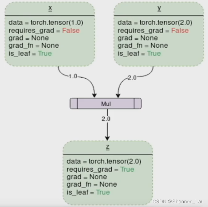
z = x ∗ y z=x*y z=x∗y
z z z是由这个操作得到的,也就是Mul(multiply)。 z z z的值就是 x ∗ y x*y x∗y的值。
因为 z z z是 x ∗ y x*y x∗y得到的,所以requires_grad=True,就是说z是可以求导的,可以对 x x x、 y y y求导
grad=None是还没求导,求导之后才知道导数和梯度是多少
grad_fn=None,函数形式是什么还不知道(因为还没有求导)
is_leaf=True 很关键,求导要知道其终点是什么时候,如果is_leaf=True,requires_grad=False就意味着到了最开始的一层,就不能再往前传了。
2.3 拓展
静态图和动态图——主要区别在于是否需要预先定义计算图的结构
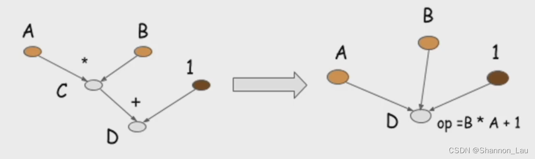
动态图不需要定义操作符。
2.4 演示
通过一个简单的函数 y = x 1 + 2 x 2 y=x_1+2x_2 y=x1+2x2来说明自动求导
x1 = torch.tensor(1.0, requires_grad=True)
x2 = torch.tensor(2.0, requires_grad=True)
y = x1 + 2 * x2
print(y)

>>>
tensor(5., grad_fn=<AddBackward0>)
# 首先查看每个变量是否需要求导
print(x1.requires_grad)
print(x2.requires_grad)
print(y.requires_grad)
>>>
True
True
True
# 查看每个变量导数的大小,此时因为没有反向传播,所以导数都不存在
print(x1.grad.data)
print(x2.grad.data)
print(y.grad.data)
>>>
---------------------------------------------------------------------------
AttributeError                            Traceback (most recent call last)
Input In [33], in <cell line: 2>()
      1 # 查看每个变量导数的大小,此时因为没有反向传播,所以导数都不存在
----> 2 print(x1.grad.data)
      3 print(x2.grad.data)
      4 print(y.grad.data)

AttributeError: 'NoneType' object has no attribute 'data'
前向传播之后是不会有导数存在的,每个节点上是不会有梯度值计入的
# 反向传播之后看导数大小
y = x1 + 2 * x2
y.backward()
print(x1.grad.data)
print(x2.grad.data)
>>>
tensor(1.)
tensor(2.)
# 导数是会累积的,重复运行相同命令,grad会增加
y = x1 + 2 * x2
y.backward()
print(x1.grad.data)
print(x2.grad.data)
>>>
tensor(2.)
tensor(4.)
所以每次计算前需要清楚当前导数值避免积累,这一功能可以通过pytorch的optimizer实现
# 尝试,如果不允许求导,会是什么样?
x1 = torch.tensor(1.0, requires_grad=False)
x2 = torch.tensor(2.0, requires_grad=False)
y = x1 + 2 * x2
y.backward()
>>>
---------------------------------------------------------------------------
RuntimeError                              Traceback (most recent call last)
Input In [39], in <cell line: 5>()
      3 x2 = torch.tensor(2.0, requires_grad=False)
      4 y = x1 + 2 * x2
----> 5 y.backward()

File ~\anaconda3\envs\pytorch\lib\site-packages\torch\_tensor.py:363, in Tensor.backward(self, gradient, retain_graph, create_graph, inputs)
    354 if has_torch_function_unary(self):
    355     return handle_torch_function(
    356         Tensor.backward,
    357         (self,),
   (...)
    361         create_graph=create_graph,
    362         inputs=inputs)
--> 363 torch.autograd.backward(self, gradient, retain_graph, create_graph, inputs=inputs)

File ~\anaconda3\envs\pytorch\lib\site-packages\torch\autograd\__init__.py:173, in backward(tensors, grad_tensors, retain_graph, create_graph, grad_variables, inputs)
    168     retain_graph = create_graph
    170 # The reason we repeat same the comment below is that
    171 # some Python versions print out the first line of a multi-line function
    172 # calls in the traceback and some print out the last line
--> 173 Variable._execution_engine.run_backward(  # Calls into the C++ engine to run the backward pass
    174     tensors, grad_tensors_, retain_graph, create_graph, inputs,
    175     allow_unreachable=True, accumulate_grad=True)

RuntimeError: element 0 of tensors does not require grad and does not have a grad_fn


 1648
1648


 被折叠的 条评论
为什么被折叠?
被折叠的 条评论
为什么被折叠?
 到【灌水乐园】发言


