特征工程——交互特征（多项式特征）

最新推荐文章于 2024-04-19 16:09:25 发布

PresleyR

最新推荐文章于 2024-04-19 16:09:25 发布

阅读量861

点赞数

本文链接：https://blog.csdn.net/PresleyR/article/details/128887929

版权

一、交互特征定义

两个特征的乘积可以组成一对简单的交互特征，这种相乘关系可以用逻辑操作符AND来类比，它可以表示出由一对条件形成的结果：“该购买行为来自于邮政编码为98121的地区”AND“用户年龄在18和35岁之间”。这种特征在基于决策树的模型中极其常见，在广义线性模型中也经常使用。

简单线性模型使用独立输入特征 $x_{1}$ , $x_{2}$ , …, $x_{n}$ 的线性组合来预测结果变量： $y=w_{1}x_{}1+w_{2}x_{2}+...+w_{n}x_{n}$ 。

很容易对线性模型进行扩展，使之包含输入特征的两两组合，如下： $y=w_{1}x_{1}+w_{2}x_{2}+...+w_{n}x_{n}+w_{1,1}x_{1}x_{1}+w_{1,2}x_{1}x_{2}+w_{1,3}x_{1}x_{3}+...$ 。

这样，就可以捕获特征之间的交互作用，因此这些特征对就称为交互特征。如果 $x_{1}$ 和<img alt="x_{2}" class="mathcode" src="https://private.codecogs.com/gif.latex?x_%7B2%7D">是二值特征，那么它们的积<img alt="x_{1}x_{2}" class="mathcode" src="https://private.codecogs.com/gif.latex?x_%7B1%7Dx_%7B2%7D">就是逻辑函数<img alt="x_{1}" class="mathcode" src="https://private.codecogs.com/gif.latex?x_%7B1%7D">&nbsp;AND <img alt="x_{2}" class="mathcode" src="https://private.codecogs.com/gif.latex?x_%7B2%7D">。如果我们的问题是基于客户档案信息来预测客户偏好，那么在这个例子中，除了根据用户的年龄<span style="color:#f33b45;">或地点这些单独特征来进行预测，还可以使用交互特征来根据用户位于某个年龄段<span style="color: #f33b45;">并且位于某个特定地点来进行预测。

二、sklearn的PolynomialFeatures的用法

使用 sklearn.preprocessing.PolynomialFeatures 这个类可以进行特征的构造，构造的方式就是特征与特征相乘(自己与自己，自己与其他人)，这种方式叫做使用多项式的方式。例如：有 $x_{0}$ 、 $x_{1}$ 两个特征，那么它的 2 次多项式的次数为 [ $1,x_{0},x_{1},x_{0}^{2},x_{0}x_{1},x_{1}^{2}$ ]。

PolynomialFeatures 这个类有 3 个参数：

degree：控制多项式的次数；
interaction_only：默认为 False，如果指定为 True，那么就不会有特征自己和自己结合的项，组合的特征中没有 $x_{0}^{2}$ 和 $x_{1}^{2}$ ；
include_bias：默认为 True 。如果为 True 的话，那么结果中就会有 0 次幂项，即全为 1 这一列。

1、案例一：多项式特征构造过程

1.1、建立数据

from sklearn.preprocessing import PolynomialFeatures

import numpy as np

X=np.arange(6).reshape(3,2)

X

输出：

array([[0, 1],

[2, 3],

[4, 5]])

1.2、设置多项式阶数为2，其他默认。

poly1=PolynomialFeatures(degree=2)

res1=poly1.fit_transform(X)

res1

输出：

array([[ 1., 0., 1., 0., 0., 1.],

[ 1., 2., 3., 4., 6., 9.],

[ 1., 4., 5., 16., 20., 25.]])
 interaction_only，默认为 False，既组合的特征中有x_{0}^{2}和x_{1}^{2}；include_bias，默认为 True，那么结果中就会有x_{0}^{0}x_{1}^{0}，即全为 1 这一列。如果interaction_only设置为True，include_bias设置为False，则会变成如下：


poly2=PolynomialFeatures(interaction_only=True,include_bias=False)

res2=poly2.fit_transform(X)

res2

输出：

array([[ 0., 1., 0.],

[ 2., 3., 6.],

[ 4., 5., 20.]])
既少了1,x_{0}^{2},x_{1}^{2}这三列。

1.3、PolynomialFeatures可返回的参数

输出转换之后的特征名称：

poly1.get_feature_names()

输出：

['1', 'x0', 'x1', 'x0^2', 'x0 x1', 'x1^2']

 我们可以输出数据的转换次数(幂)：


#输出6个特征，来自原来的2个特征的幂(转变过程)

poly1.powers_

输出：

array([[0, 0],

[1, 0],

[0, 1],

[2, 0],

[1, 1],

[0, 2]], dtype=int64)
 其中：

[0,0]表示新特征由原始特征这样组成：x_{0}^{0}\cdot x_{1}^{0}，其实就是1这一列；

[1,0]表示新特征由原始特征这样组成：x_{0}^{1}\cdot x_{1}^{0}，其实就是阿x_{0}这一列；

[0,1]表示新特征由原始特征这样组成：x_{0}^{0}\cdot x_{1}^{1}，其实就是x_{1}这一列；

[2,0]表示新特征由原始特征这样组成：x_{0}^{2}\cdot x_{1}^{0}，其实就是x_{0}^{2}这一列；

[1,1]表示新特征由原始特征这样组成：x_{0}^{1}\cdot x_{1}^{1}，其实就是x_{0}\cdot x_{1}这一列；

[0,2]表示新特征由原始特征这样组成：x_{0}^{0}\cdot x_{1}^{2}，其实就是x_{1}^{2}这一列；

同样，我们可以输出转换前后的特征个数：


#输出原始特征个数

poly1.n_input_features_



#输出多项式转换之后的特征个数

poly1.n_output_features_

输出：

2、案例二：多项式特征应用于回归模型

2.1、建立数据

from sklearn.linear_model import LinearRegression

from sklearn.tree import DecisionTreeRegressor

from sklearn.preprocessing import PolynomialFeatures

import mglearn

import numpy as np

import matplotlib.pyplot as plt



#建立数据

X, y = mglearn.datasets.make_wave(n_samples=100) #100个样本点

X.shape



y.shape



#辅助数据，用于绘制回归曲线

line = np.linspace(-3, 3, 1000, endpoint=False).reshape(-1, 1)

line.shape

输出：

(100, 1)



(100,)



(1000, 1)

2.2、构造多项式特征

#包含到x^10的多项式

#默认的include_bias=True添加恒等于1的常数特征

poly = PolynomialFeatures(degree=10, include_bias=False)

poly.fit(X)

X_poly = poly.transform(X)

X_poly.shape



poly.get_feature_names()



X_poly[:5]



X[:5]

输出：

(100, 10)



['x0', 'x0^2', 'x0^3', 'x0^4', 'x0^5', 'x0^6', 'x0^7', 'x0^8', 'x0^9', 'x0^10']



array([[-7.52759287e-01, 5.66646544e-01, -4.26548448e-01,

3.21088306e-01, -2.41702204e-01, 1.81943579e-01,

-1.36959719e-01, 1.03097700e-01, -7.76077513e-02,

5.84199555e-02],

[ 2.70428584e+00, 7.31316190e+00, 1.97768801e+01,

5.34823369e+01, 1.44631526e+02, 3.91124988e+02,

1.05771377e+03, 2.86036036e+03, 7.73523202e+03,

2.09182784e+04],

[ 1.39196365e+00, 1.93756281e+00, 2.69701700e+00,

3.75414962e+00, 5.22563982e+00, 7.27390068e+00,

1.01250053e+01, 1.40936394e+01, 1.96178338e+01,

2.73073115e+01],

[ 5.91950905e-01, 3.50405874e-01, 2.07423074e-01,

1.22784277e-01, 7.26822637e-02, 4.30243318e-02,

2.54682921e-02, 1.50759786e-02, 8.92423917e-03,

5.28271146e-03],

[-2.06388816e+00, 4.25963433e+00, -8.79140884e+00,

1.81444846e+01, -3.74481869e+01, 7.72888694e+01,

-1.59515582e+02, 3.29222321e+02, -6.79478050e+02,

1.40236670e+03]])



array([[-0.75275929],

[ 2.70428584],

[ 1.39196365],

[ 0.59195091],

[-2.06388816]])

 从上面我们可以得出，多项式特征的构成过程为[x_{0}]\rightarrow [x_{0},x_{0}^{2},x_{0}^{3},x_{0}^{4},x_{0}^{5},x_{0}^{6},x_{0}^{7},x_{0}^{8},x_{0}^{9},x_{0}^{10}]，从1列变成了10列。

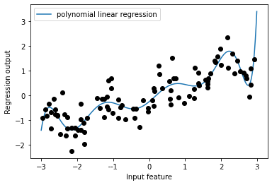
2.3、回归模型训练及可视化

将多项式特征与回归模型一起使用，可以得到经典的多项式回归。

reg = LinearRegression().fit(X_poly, y)



line_poly = poly.transform(line)

plt.plot(line, reg.predict(line_poly), label='polynomial linear regression')

plt.plot(X[:, 0], y, 'o', c='k')

plt.ylabel("Regression output")

plt.xlabel("Input feature")

plt.legend(loc="best")

输出：

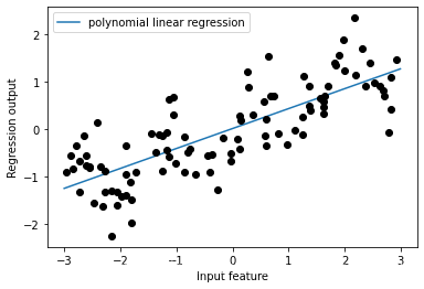
原始没有进行转换的数据，结合回归模型，得到的是简单的线性回归模型。

reg = LinearRegression().fit(X, y)



line_poly = poly.transform(line)

plt.plot(line, reg.predict(line), label='linear regression')

plt.plot(X[:, 0], y, 'o', c='k')

plt.ylabel("Regression output")

plt.xlabel("Input feature")

plt.legend(loc="best")

输出：

作为对比，下面用较复杂的模型——核SVM模型来学习原始数据，原数据没有做任何变换。

from sklearn.svm import SVR



for gamma in [1, 10]:

svr = SVR(gamma=gamma).fit(X, y)

plt.plot(line, svr.predict(line), label='SVR gamma={}'.format(gamma))



plt.plot(X[:, 0], y, 'o', c='k')

plt.ylabel("Regression output")

plt.xlabel("Input feature")

plt.legend(loc="best")

输出：

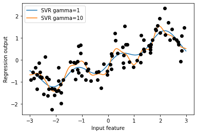
以上我们可以得到：使用更为复杂的模型(如核SVM)，且不需要进行显式地特征变换，我们也能够学习到一个与多项式回归(简单回归+多项式特征转换)复杂度类似的预测结果。

3、案例三：NFL原则讨论

3.1、采用波士顿房价数据集，利用MinMaxScaler将其放缩到0-1之间

from sklearn.datasets import load_boston

from sklearn.model_selection import train_test_split

from sklearn.preprocessing import MinMaxScaler



boston = load_boston()

X_train, X_test, y_train, y_test = train_test_split(

boston.data, boston.target, random_state=0)



# MinMaxScaler

scaler = MinMaxScaler()

X_train_scaled = scaler.fit_transform(X_train)

X_test_scaled = scaler.transform(X_test)

3.2、提取多项式特征和交互特征

poly = PolynomialFeatures(degree=2).fit(X_train_scaled)

X_train_poly = poly.transform(X_train_scaled)

X_test_poly = poly.transform(X_test_scaled)

print("X_train.shape: {}".format(X_train.shape))

print("X_train_poly.shape: {}".format(X_train_poly.shape))

print("Polynomial feature names:\n{}".format(poly.get_feature_names()))

输出：

X_train.shape: (379, 13)



X_train_poly.shape: (379, 105)



Polynomial feature names:

['1', 'x0', 'x1', 'x2', 'x3', 'x4', 'x5', 'x6', 'x7', 'x8', 'x9', 'x10', 'x11', 'x12', 'x0^2', 'x0 x1', 'x0 x2', 'x0 x3', 'x0 x4', 'x0 x5', 'x0 x6', 'x0 x7', 'x0 x8', 'x0 x9', 'x0 x10', 'x0 x11', 'x0 x12', 'x1^2', 'x1 x2', 'x1 x3', 'x1 x4', 'x1 x5', 'x1 x6', 'x1 x7', 'x1 x8', 'x1 x9', 'x1 x10', 'x1 x11', 'x1 x12', 'x2^2', 'x2 x3', 'x2 x4', 'x2 x5', 'x2 x6', 'x2 x7', 'x2 x8', 'x2 x9', 'x2 x10', 'x2 x11', 'x2 x12', 'x3^2', 'x3 x4', 'x3 x5', 'x3 x6', 'x3 x7', 'x3 x8', 'x3 x9', 'x3 x10', 'x3 x11', 'x3 x12', 'x4^2', 'x4 x5', 'x4 x6', 'x4 x7', 'x4 x8', 'x4 x9', 'x4 x10', 'x4 x11', 'x4 x12', 'x5^2', 'x5 x6', 'x5 x7', 'x5 x8', 'x5 x9', 'x5 x10', 'x5 x11', 'x5 x12', 'x6^2', 'x6 x7', 'x6 x8', 'x6 x9', 'x6 x10', 'x6 x11', 'x6 x12', 'x7^2', 'x7 x8', 'x7 x9', 'x7 x10', 'x7 x11', 'x7 x12', 'x8^2', 'x8 x9', 'x8 x10', 'x8 x11', 'x8 x12', 'x9^2', 'x9 x10', 'x9 x11', 'x9 x12', 'x10^2', 'x10 x11', 'x10 x12', 'x11^2', 'x11 x12', 'x12^2']

3.3、对Ridge(岭回归)在有交互特征地数据集和没有交互特征地数据上地性能进行对比

from sklearn.linear_model import Ridge

ridge = Ridge().fit(X_train_scaled, y_train)

print("Score without interactions: {:.3f}".format(

ridge.score(X_test_scaled, y_test)))

ridge = Ridge().fit(X_train_poly, y_train)

print("Score with interactions: {:.3f}".format(

ridge.score(X_test_poly, y_test)))

输出：

Score without interactions: 0.621

Score with interactions: 0.753

显然，在使用Ridge(岭回归)时，交互特征和多项式特征对性能有很大地提升。但如果使用更复杂地模型(比如随机森林)，情况可能会稍有不同。如下：

from sklearn.ensemble import RandomForestRegressor

rf = RandomForestRegressor(n_estimators=100).fit(X_train_scaled, y_train)

print("Score without interactions: {:.3f}".format(

rf.score(X_test_scaled, y_test)))

rf = RandomForestRegressor(n_estimators=100).fit(X_train_poly, y_train)

print("Score with interactions: {:.3f}".format(rf.score(X_test_poly, y_test)))

输出：

Score without interactions: 0.807

Score with interactions: 0.777

可以看出，即使没有额外的特征，随机森林的性能也要优于Ridge(岭回归)。添加交互项特征和多项式特征实际上会略微降低其性能。关于此方面问题，大家想深入了解的话，可见《 NFL定理》。

PresleyR

关注

0
点赞
踩
7

收藏

觉得还不错? 一键收藏
0
评论
特征工程——交互特征（多项式特征）

一、交互特征定义两个特征的乘积可以组成一对简单的交互特征，这种相乘关系可以用逻辑操作符AND来类比，它可以表示出由一对条件形成的结果：“该购买行为来自于邮政编码为98121的地区”AND“用户年龄在18和35岁之间”。这种特征在基于决策树的模型中极其常见，在广义线性模型中也经常使用。简单线性模型使用独立输入特征, , …, 的线性组合来预测结果变量：。很容易对线性模型进行扩展，使之包含输...
复制链接

扫一扫