


这个项目包含了吴恩达机器学习ex2的python实现,主要知识点为逻辑回归、正则化,题目内容可以查看数据集中的ex2.pdf
代码来自网络(原作者黄广海的github),添加了部分对于题意的中文翻译,以及修改成与习题一致的结构,方便大家理解
另,原来代码中的高次项有些问题,以及缺少作图部分,已经修改补全
其余练习的传送门
1 逻辑回归
在训练的初始阶段,我们将要构建一个逻辑回归模型来预测,某个学生是否被大学录取。
设想你是大学相关部分的管理者,想通过申请学生两次测试的评分,来决定他们是否被录取。
现在你拥有之前申请学生的可以用于训练逻辑回归的训练样本集。对于每一个训练样本,你有他们两次测试的评分和最后是被录取的结果。
1.1 数据可视化
import numpy as np
import pandas as pd
import matplotlib.pyplot as plt
path = '/home/kesci/input/andrew_ml_ex22391/ex2data1.txt'
data = pd.read_csv(path, header=None, names=['Exam 1', 'Exam 2', 'Admitted'])
data.head()
positive = data[data['Admitted'].isin([1])]
negative = data[data['Admitted'].isin([0])]

fig, ax = plt.subplots(figsize=(12,8))
ax.scatter(positive['Exam 1'], positive['Exam 2'], s=50, c='b', marker='o', label='Admitted')
ax.scatter(negative['Exam 1'], negative['Exam 2'], s=50, c='r', marker='x', label='Not Admitted')
ax.legend()
ax.set_xlabel('Exam 1 Score')
ax.set_ylabel('Exam 2 Score')
plt.show()

1.2 实现
1.2.1 sigmoid 函数
逻辑回归函数为
g代表一个常用的逻辑函数(logistic function)为S形函数(Sigmoid function),公式为:
合起来,我们得到逻辑回归模型的假设函数:
# 实现sigmoid函数
def sigmoid(z):
    return 1 / (1 + np.exp(-z))
1.2.2 代价函数和梯度
代价函数:
梯度:
虽然这个梯度和前面线性回归的梯度很像,但是要记住$h_\theta(x)$是不一样的
实现完成后,用初始$\theta$代入计算,结果应该是0.693左右
# 实现代价函数
def cost(theta, X, y):
    theta = np.matrix(theta)
    X = np.matrix(X)
    y = np.matrix(y)
    first = np.multiply(-y, np.log(sigmoid(X * theta.T)))
    second = np.multiply((1 - y), np.log(1 - sigmoid(X * theta.T)))
    return np.sum(first - second) / (len(X))
初始化X,y,$\theta$
# 加一列常数列
data.insert(0, 'Ones', 1)

# 初始化X,y,θ
cols = data.shape[1]
X = data.iloc[:,0:cols-1]
y = data.iloc[:,cols-1:cols]
theta = np.zeros(3)

# 转换X,y的类型
X = np.array(X.values)
y = np.array(y.values)
# 检查矩阵的维度
X.shape, theta.shape, y.shape
# 用初始θ计算代价
cost(theta, X, y)
# 实现梯度计算的函数(并没有更新θ)
def gradient(theta, X, y):
    theta = np.matrix(theta)
    X = np.matrix(X)
    y = np.matrix(y)

    parameters = int(theta.ravel().shape[1])
    grad = np.zeros(parameters)

    error = sigmoid(X * theta.T) - y

    for i in range(parameters):
        term = np.multiply(error, X[:,i])
        grad[i] = np.sum(term) / len(X)

    return grad
1.2.3 用工具库计算θ的值
在此前的线性回归中,我们自己写代码实现的梯度下降(ex1的2.2.4的部分)。当时我们写了一个代价函数、计算了他的梯度,然后对他执行了梯度下降的步骤。这次,我们不自己写代码实现梯度下降,我们会调用一个已有的库。这就是说,我们不用自己定义迭代次数和步长,功能会直接告诉我们最优解。
andrew ng在课程中用的是Octave的“fminunc”函数,由于我们使用Python,我们可以用scipy.optimize.fmin_tnc做同样的事情。
(另外,如果对fminunc有疑问的,可以参考下面这篇百度文库的内容https://wenku.baidu.com/view/2f6ce65d0b1c59eef8c7b47a.html )
如果一切顺利的话,最有θ对应的代价应该是0.203
import scipy.optimize as opt
result = opt.fmin_tnc(func=cost, x0=theta, fprime=gradient, args=(X, y))
result
让我们看看在这个结论下代价函数计算结果是什么个样子~
# 用θ的计算结果代回代价函数计算
cost(result[0], X, y)
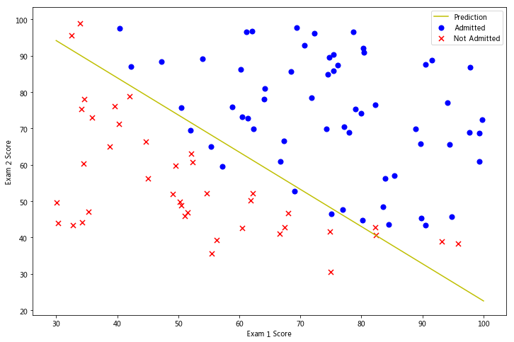
画出决策曲线
plotting_x1 = np.linspace(30, 100, 100)
plotting_h1 = ( - result[0][0] - result[0][1] * plotting_x1) / result[0][2]

fig, ax = plt.subplots(figsize=(12,8))
ax.plot(plotting_x1, plotting_h1, 'y', label='Prediction')
ax.scatter(positive['Exam 1'], positive['Exam 2'], s=50, c='b', marker='o', label='Admitted')
ax.scatter(negative['Exam 1'], negative['Exam 2'], s=50, c='r', marker='x', label='Not Admitted')
ax.legend()
ax.set_xlabel('Exam 1 Score')
ax.set_ylabel('Exam 2 Score')
plt.show()
1.2.4 评价逻辑回归模型
在确定参数之后,我们可以使用这个模型来预测学生是否录取。如果一个学生exam1得分45,exam2得分85,那么他录取的概率应为0.776
# 实现hθ
def hfunc1(theta, X):
    return sigmoid(np.dot(theta.T, X))
hfunc1(result[0],[1,45,85])
另一种评价θ的方法是看模型在训练集上的正确率怎样。写一个predict的函数,给出数据以及参数后,会返回“1”或者“0”。然后再把这个predict函数用于训练集上,看准确率怎样。
# 定义预测函数
def predict(theta, X):
    probability = sigmoid(X * theta.T)
    return [1 if x >= 0.5 else 0 for x in probability]
# 统计预测正确率
theta_min = np.matrix(result[0])
predictions = predict(theta_min, X)
correct = [1 if ((a == 1 and b == 1) or (a == 0 and b == 0)) else 0 for (a, b) in zip(predictions, y)]
accuracy = (sum(map(int, correct)) % len(correct))
print ('accuracy = {0}%'.format(accuracy))
画出对应曲线
2 正则化逻辑回归
在训练的第二部分,我们将实现加入正则项提升逻辑回归算法。
设想你是工厂的生产主管,你有一些芯片在两次测试中的测试结果,测试结果决定是否芯片要被接受或抛弃。你有一些历史数据,帮助你构建一个逻辑回归模型。
2.1 数据可视化
path =  '/home/kesci/input/andrew_ml_ex22391/ex2data2.txt'
data_init = pd.read_csv(path, header=None, names=['Test 1', 'Test 2', 'Accepted'])
data_init.head()
positive2 = data_init[data_init['Accepted'].isin([1])]
negative2 = data_init[data_init['Accepted'].isin([0])]

fig, ax = plt.subplots(figsize=(12,8))
ax.scatter(positive2['Test 1'], positive2['Test 2'], s=50, c='b', marker='o', label='Accepted')
ax.scatter(negative2['Test 1'], negative2['Test 2'], s=50, c='r', marker='x', label='Rejected')
ax.legend()
ax.set_xlabel('Test 1 Score')
ax.set_ylabel('Test 2 Score')
plt.show()
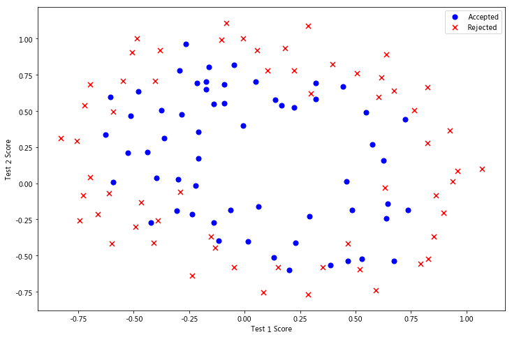
以上图片显示,这个数据集不能像之前一样使用直线将两部分分割。而逻辑回归只适用于线性的分割,所以,这个数据集不适合直接使用逻辑回归。
2.2 特征映射
一种更好的使用数据集的方式是为每组数据创造更多的特征。所以我们为每组$x_1,x_2$添加了最高到6次幂的特征
degree = 6
data2 = data_init
x1 = data2['Test 1']
x2 = data2['Test 2']

data2.insert(3, 'Ones', 1)

for i in range(1, degree+1):
    for j in range(0, i+1):
        data2['F' + str(i-j) + str(j)] = np.power(x1, i-j) * np.power(x2, j)
#此处原答案错误较多,已经更正

data2.drop('Test 1', axis=1, inplace=True)
data2.drop('Test 2', axis=1, inplace=True)

data2.head()
3.2 代价函数和梯度
这一部分要实现计算逻辑回归的代价函数和梯度的函数。代价函数公式如下:
记住$\theta_0$是不需要正则化的,下标从1开始。
梯度的第j个元素的更新公式为:
对上面的算法中 j=1,2,...,n 时的更新式子进行调整可得:
把初始$\theta$(所有元素为0)带入,代价应为0.693
# 实现正则化的代价函数
def costReg(theta, X, y, learningRate):
    theta = np.matrix(theta)
    X = np.matrix(X)
    y = np.matrix(y)
    first = np.multiply(-y, np.log(sigmoid(X * theta.T)))
    second = np.multiply((1 - y), np.log(1 - sigmoid(X * theta.T)))
    reg = (learningRate / (2 * len(X))) * np.sum(np.power(theta[:,1:theta.shape[1]], 2))
    return np.sum(first - second) / len(X) + reg
# 实现正则化的梯度函数
def gradientReg(theta, X, y, learningRate):
    theta = np.matrix(theta)
    X = np.matrix(X)
    y = np.matrix(y)

    parameters = int(theta.ravel().shape[1])
    grad = np.zeros(parameters)

    error = sigmoid(X * theta.T) - y

    for i in range(parameters):
        term = np.multiply(error, X[:,i])

        if (i == 0):
            grad[i] = np.sum(term) / len(X)
        else:
            grad[i] = (np.sum(term) / len(X)) + ((learningRate / len(X)) * theta[:,i])

    return grad
# 初始化X,y,θ
cols = data2.shape[1]
X2 = data2.iloc[:,1:cols]
y2 = data2.iloc[:,0:1]
theta2 = np.zeros(cols-1)

# 进行类型转换
X2 = np.array(X2.values)
y2 = np.array(y2.values)

# λ设为1
learningRate = 1
# 计算初始代价
costReg(theta2, X2, y2, learningRate)
2.3.1 用工具库求解参数
result2 = opt.fmin_tnc(func=costReg, x0=theta2, fprime=gradientReg, args=(X2, y2, learningRate))
result2
最后,我们可以使用第1部分中的预测函数来查看我们的方案在训练数据上的准确度。
theta_min = np.matrix(result2[0])
predictions = predict(theta_min, X2)
correct = [1 if ((a == 1 and b == 1) or (a == 0 and b == 0)) else 0 for (a, b) in zip(predictions, y2)]
accuracy = (sum(map(int, correct)) % len(correct))
print ('accuracy = {0}%'.format(accuracy))
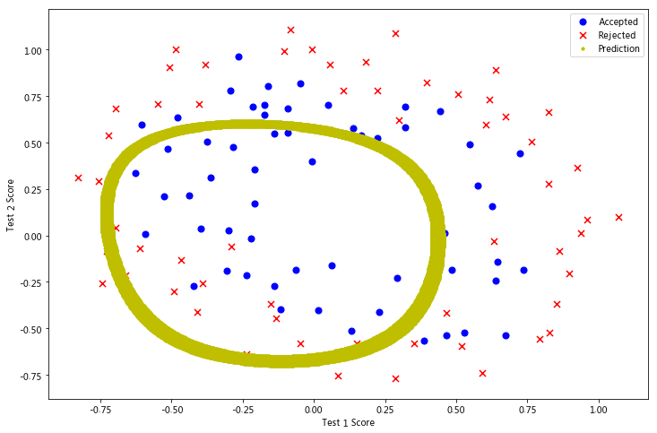
2.4 画出决策的曲线
def hfunc2(theta, x1, x2):
    temp = theta[0][0]
    place = 0
    for i in range(1, degree+1):
        for j in range(0, i+1):
            temp+= np.power(x1, i-j) * np.power(x2, j) * theta[0][place+1]
            place+=1
    return temp
def find_decision_boundary(theta):
    t1 = np.linspace(-1, 1.5, 1000)
    t2 = np.linspace(-1, 1.5, 1000)

    cordinates = [(x, y) for x in t1 for y in t2]
    x_cord, y_cord = zip(*cordinates)
    h_val = pd.DataFrame({'x1':x_cord, 'x2':y_cord})
    h_val['hval'] = hfunc2(theta, h_val['x1'], h_val['x2'])

    decision = h_val[np.abs(h_val['hval']) < 2 * 10**-3]
    return decision.x1, decision.x2
fig, ax = plt.subplots(figsize=(12,8))
ax.scatter(positive2['Test 1'], positive2['Test 2'], s=50, c='b', marker='o', label='Accepted')
ax.scatter(negative2['Test 1'], negative2['Test 2'], s=50, c='r', marker='x', label='Rejected')
ax.set_xlabel('Test 1 Score')
ax.set_ylabel('Test 2 Score')

x, y = find_decision_boundary(result2)
plt.scatter(x, y, c='y', s=10, label='Prediction')
ax.legend()
plt.show()

2.5 改变λ,观察决策曲线
$\lambda=0$时过拟合
learningRate2 = 0
result3 = opt.fmin_tnc(func=costReg, x0=theta2, fprime=gradientReg, args=(X2, y2, learningRate2))
fig, ax = plt.subplots(figsize=(12,8))
ax.scatter(positive2['Test 1'], positive2['Test 2'], s=50, c='b', marker='o', label='Accepted')
ax.scatter(negative2['Test 1'], negative2['Test 2'], s=50, c='r', marker='x', label='Rejected')
ax.set_xlabel('Test 1 Score')
ax.set_ylabel('Test 2 Score')

x, y = find_decision_boundary(result3)
plt.scatter(x, y, c='y', s=10, label='Prediction')
ax.legend()
plt.show()

$\lambda=100$时欠拟合
learningRate3 = 100
result4 = opt.fmin_tnc(func=costReg, x0=theta2, fprime=gradientReg, args=(X2, y2, learningRate3))
fig, ax = plt.subplots(figsize=(12,8))
ax.scatter(positive2['Test 1'], positive2['Test 2'], s=50, c='b', marker='o', label='Accepted')
ax.scatter(negative2['Test 1'], negative2['Test 2'], s=50, c='r', marker='x', label='Rejected')
ax.set_xlabel('Test 1 Score')
ax.set_ylabel('Test 2 Score')

x, y = find_decision_boundary(result4)
plt.scatter(x, y, c='y', s=10, label='Prediction')
ax.legend()
plt.show()


 4226
4226


 被折叠的 条评论
为什么被折叠?
被折叠的 条评论
为什么被折叠?
 到【灌水乐园】发言


