《图算法》第八章用图算法增强机器学习-3

最新推荐文章于 2020-05-20 19:58:56 发布

ifeng0310

最新推荐文章于 2020-05-20 19:58:56 发布

阅读量417

点赞数

分类专栏：图算法文章标签：图算法图数据库 neo4j

原文链接：https://mp.weixin.qq.com/s/2i3k0hJjfnb3Npn5hYhDDw

版权

图算法专栏收录该内容

20 篇文章 18 订阅

订阅专栏

对图算法有兴趣的朋友可以关注微信公众号：《 Medical与AI的故事》

原文链接：《图算法》第八章-3 用图算法增强机器学习

如何评估结果

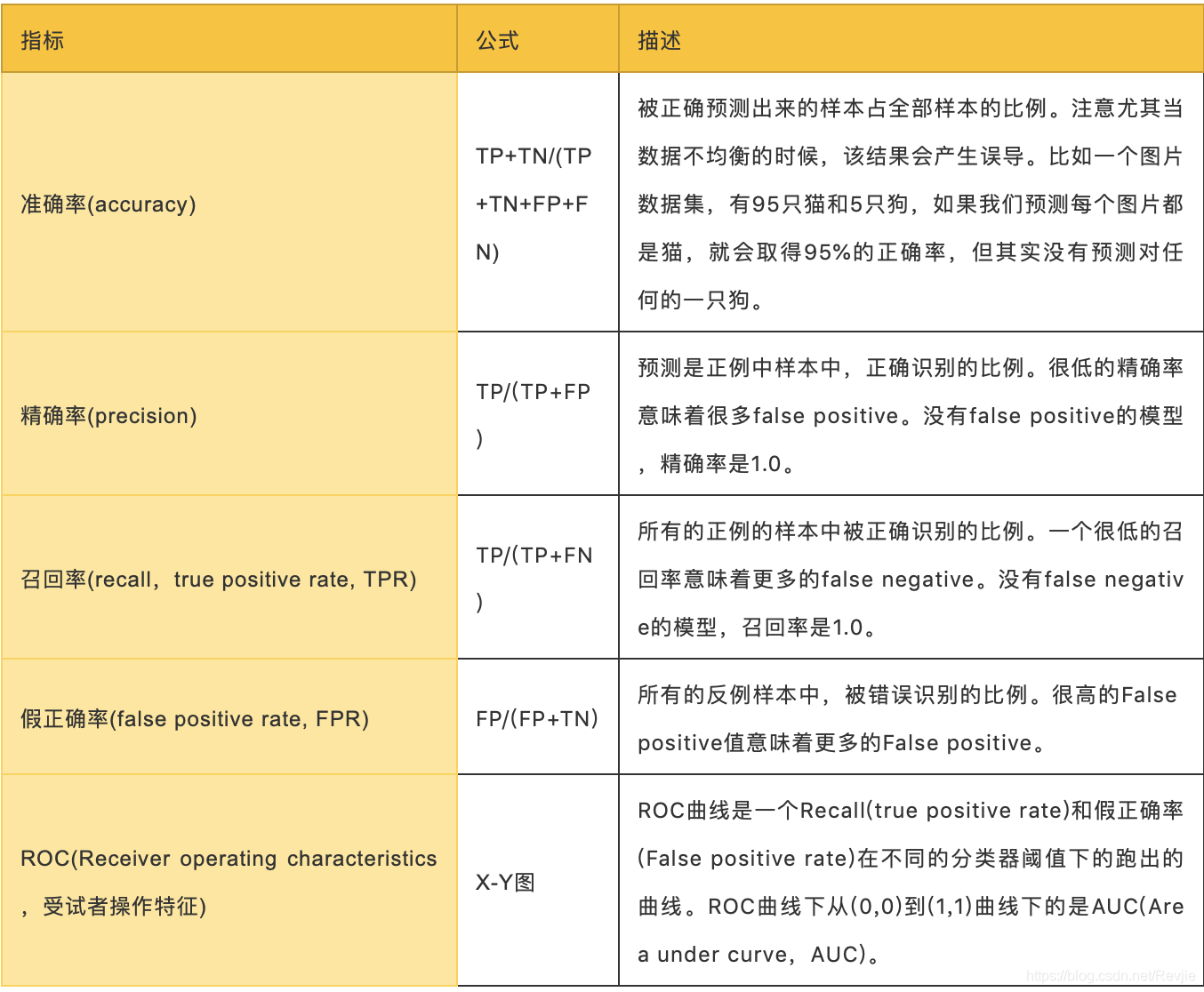
现在让我们根据测试集评估我们的模型。尽管有几种方法可以评估模型的性能，但大多数方法都是根据一些基线预测指标得出的，如表8-1所示：
表8-1.预测指标
在这里插入图片描述
其中，对于TP，FN，FP，TN的解释如下：

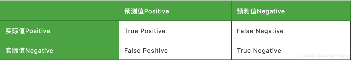
对于二元分类，根据实际值和预测值的关系，共有四种分类：True Positive, True Negative, False Negative, False Positive。它们的格式：(预测值==实际值) 预测值。比如False Negative指的是预测分类是Negative，实际分类是Positive，所以预测正确与否是False。

ROC曲线：对于数据集，如果设置从0开始逐渐增大的概率阈值，意味着越来越多的样本被划分成为正例。在每一个阈值下，都得到一组（FPR，TPR）。最终可以形成曲线，叫做ROC，受试者操作特征。

我们将使用准确度（accuracy）、精确率（precision）、召回率（recall）和ROC曲线来评估我们的模型。准确度是一个粗略的度量，所以我们将重点提高我们的整体精度和召回度。我们将使用ROC曲线比较各个特征如何改变预测率。

根据我们的目标，我们可能希望采用不同的措施。例如，我们可能想消除所有疾病指标的假阴性（false negative），但我们不想把所有的预测都推到positive的结果中。对于不同的模型，我们可能会设置多个阈值，这些阈值将一些结果传递给对错误结果的再次似然检查。

降低分类阈值会导致更全面的positive结果，从而增加false positive和true positive。

让我们使用以下函数来计算这些预测指标：

def evaluate_model(model, test_data):
    # Execute the model against the test set
    predictions = model.transform(test_data)
    # Compute true positive, false positive, false negative counts
    tp = predictions[(predictions.label == 1) &
                        (predictions.prediction == 1)].count()
    fp = predictions[(predictions.label == 0) &
                        (predictions.prediction == 1)].count()
    fn = predictions[(predictions.label == 1) &
                        (predictions.prediction == 0)].count()
    # Compute recall and precision manually
    recall = float(tp) / (tp + fn)
    precision = float(tp) / (tp + fp)
    # Compute accuracy using Spark MLLib's binary classification evaluator
    accuracy = BinaryClassificationEvaluator().evaluate(predictions)
    # Compute false positive rate and true positive rate using sklearn functions
    labels = [row["label"] for row in predictions.select("label").collect()]
    preds = [row["probability"][1] for row in predictions.select
            ("probability").collect()]
    fpr, tpr, threshold = roc_curve(labels, preds)
    roc_auc = auc(fpr, tpr)
    return { "fpr": fpr, "tpr": tpr, "roc_auc": roc_auc, "accuracy": accuracy,
                "recall": recall, "precision": precision }

然后我们将编写一个函数，以更易于使用的格式显示结果：

def display_results(results):
    results = {k: v for k, v in results.items() if k not in
                        ["fpr", "tpr", "roc_auc"]}
return pd.DataFrame({"Measure": list(results.keys()),
                        "Score": list(results.values())})

我们可以使用此代码调用函数并显示结果：

basic_results = evaluate_model(basic_model, test_data)
display_results(basic_results)

常用作者模型的预测措施有：

+-----------+----------+
| measure   | score    |
+-----------+----------+
| accuracy  | 0.864457 |
| recall    | 0.753278 |
| precision | 0.968670 |
+-----------+----------+

这不是一个糟糕的开始，因为我们预测未来的合作只基于我们两个作者中的共同作者的数量。然而，如果我们把这些措施放在一起考虑的话，我们会得到一个更大的图景。例如，该模型的精度为0.968670，这意味着它非常擅长预测链接的存在。然而，我们的召回率是0.753278，这意味着它不善于预测何时链接不存在。

我们还可以使用以下函数绘制ROC曲线（true positive和false positive的相关性图）：

def create_roc_plot():
    plt.style.use('classic')
    fig = plt.figure(figsize=(13, 8))
    plt.xlim([0, 1])
    plt.ylim([0, 1])
    plt.ylabel('True Positive Rate')
    plt.xlabel('False Positive Rate')
    plt.rc('axes', prop_cycle=(cycler('color',
                    ['r', 'g', 'b', 'c', 'm', 'y', 'k'])))
    plt.plot([0, 1], [0, 1], linestyle='--', label='Random score
                    (AUC = 0.50)')
    return plt, fig
def add_curve(plt, title, fpr, tpr, roc):
    plt.plot(fpr, tpr, label=f"{title} (AUC = {roc:0.2})”)

我们这样来调用它：

plt, fig = create_roc_plot()
add_curve(plt, "Common Authors",
                basic_results["fpr"], basic_results["tpr"], basic_results["roc_auc"])
plt.legend(loc='lower right')
plt.show()

我们可以在图8-9中看到基本模型的ROC曲线。
在这里插入图片描述
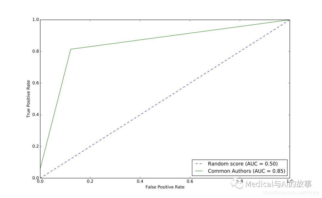
图8-9.基本模型的ROC曲线

常用作者模型给出曲线下0.86面积（AUC）评分。虽然这为我们提供了一个全面的预测指标，但我们需要图表（或其他指标）来评估这是否符合我们的目标。在图8-9中，我们看到当我们接近80%的true positive率时，我们的false positive率达到了大约20%。这在欺诈检测这样的情况下可能会有问题，在这些场景下，追查false positive的成本很高。

现在让我们使用其他的图表功能来看看我们是否可以改进我们的预测。在训练我们的模型之前，让我们看看数据是如何分布的。我们可以运行以下代码来显示每个图形功能的描述性统计信息：

(training_data.filter(training_data["label"]==1)
.describe()
.select("summary", "commonAuthors", "prefAttachment", "totalNeighbors")
.show())
(training_data.filter(training_data["label"]==0)
.describe()
.select("summary", "commonAuthors", "prefAttachment", "totalNeighbors")
.show())

我们可以在下表中看到运行这些代码位的结果：

+---------+--------------------+--------------------+--------------------+
| summary | commonAuthors      | prefAttachment     | totalNeighbors     |
+---------+--------------------+--------------------+--------------------+
| count   | 81096              | 81096              | 81096              |
| mean    | 3.5959233501035808 | 69.93537289138798  | 10.082408503502021 |
| stddev  | 4.715942231635516  | 171.47092255919472 | 8.44109970920685   |
| min     | 0                  | 1                  | 2                  |
| max     | 44                 | 3150               | 90                 |
+---------+--------------------+--------------------+——————————+


+---------+---------------------+-------------------+--------------------+
| summary | commonAuthors       | prefAttachment    | totalNeighbors     |
+---------+---------------------+-------------------+--------------------+
| count   | 81096               | 81096             | 81096              |
| mean    | 0.37666469369635985 | 48.18137762651672 | 12.97586810693499  |
| stddev  | 0.6194576095461857  | 94.92635344980489 | 10.082991078685803 |
| min     | 0                   | 1                 | 1                  |
| max     | 9                   | 1849              | 89                 |
+---------+---------------------+-------------------+--------------------+

链接（合著关系）和无链接（无合著关系）之间差异较大的功能应该更具预测性，因为两者之间的差距更大。prefAttachment的平均值对于合作过的作者比没有合作过的作者更高，这一差异在commonAuthors上更为显著。我们注意到totalNeighbors的值没有太大的差别，这可能意味着这个特征不能很好地预测。还有一个有趣的问题是prefAttachment的标准偏差大，以及它的最大值和最小值。这正是我们对具有集中集线器（超级连接者，superconnetors）的小世界网络的期望。

现在，让我们运行以下代码，来训练一个新的模型（graphy model），添加preferential attachment 和 total union of neighbors：

fields = ["commonAuthors", "prefAttachment", "totalNeighbors"]
graphy_model = train_model(fields, training_data)

让我们评估一下这个模型，并显示结果：

graphy_results = evaluate_model(graphy_model, test_data)
display_results(graphy_results)

该模型（graphy model）的预测措施如下：

+-----------+----------+
| measure   | score    |
+-----------+----------+
| accuracy  | 0.978351 |
| recall    | 0.924226 |
| precision | 0.943795 |
+-----------+----------+

我们的准确度（accuracy）和召回率（recall）大大提高了，但是准确度下降了一点，我们仍然错误地分类了大约8%的链接。让我们绘制ROC曲线，并通过运行以下代码比较基本模型和图形模型：

plt, fig = create_roc_plot()
add_curve(plt, "Common Authors",
            basic_results["fpr"], basic_results["tpr"],
            basic_results["roc_auc"])
add_curve(plt, "Graphy",
            graphy_results["fpr"], graphy_results["tpr"],
            graphy_results["roc_auc"])
plt.legend(loc='lower right')
plt.show()

我们可以在图8-10中看到输出。
在这里插入图片描述
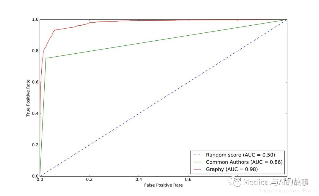
图8-10.graphy模型的ROC曲线

总的来说，我们似乎朝着正确的方向前进。可视化比较有助于这个，并了解不同的模型如何影响我们的结果。

现在我们有了多个特征，我们要评估哪些特征产生的差异最大。我们将使用特征重要性对不同特征对模型预测的影响进行排序。这使我们能够评估不同算法和统计数据对结果的影响。
在这里插入图片描述
为了计算特征重要性，Spark中的随机森林算法平均减少森林中所有树的杂质。杂质是随机分配标签错误的频率。

特征排名（feature rankings）是我们正在评估的一组特征进行比较，总是归一化为1。如果我们将一个特征排序，它的特征重要性是1.0，因为它对模型有100%的影响。

以下函数创建了一个图表，其中显示了最具影响力的功能：

def plot_feature_importance(fields, feature_importances):
    df = pd.DataFrame({"Feature": fields, "Importance": feature_importances})
    df = df.sort_values("Importance", ascending=False)
    ax = df.plot(kind='bar', x='Feature', y='Importance', legend=None)
    ax.xaxis.set_label_text("")
    plt.tight_layout()
    plt.show()

我们这样调用它：

rf_model = graphy_model.stages[-1]
plot_feature_importance(fields, rf_model.featureImportances)

运行该函数的结果如图8-11所示。
在这里插入图片描述
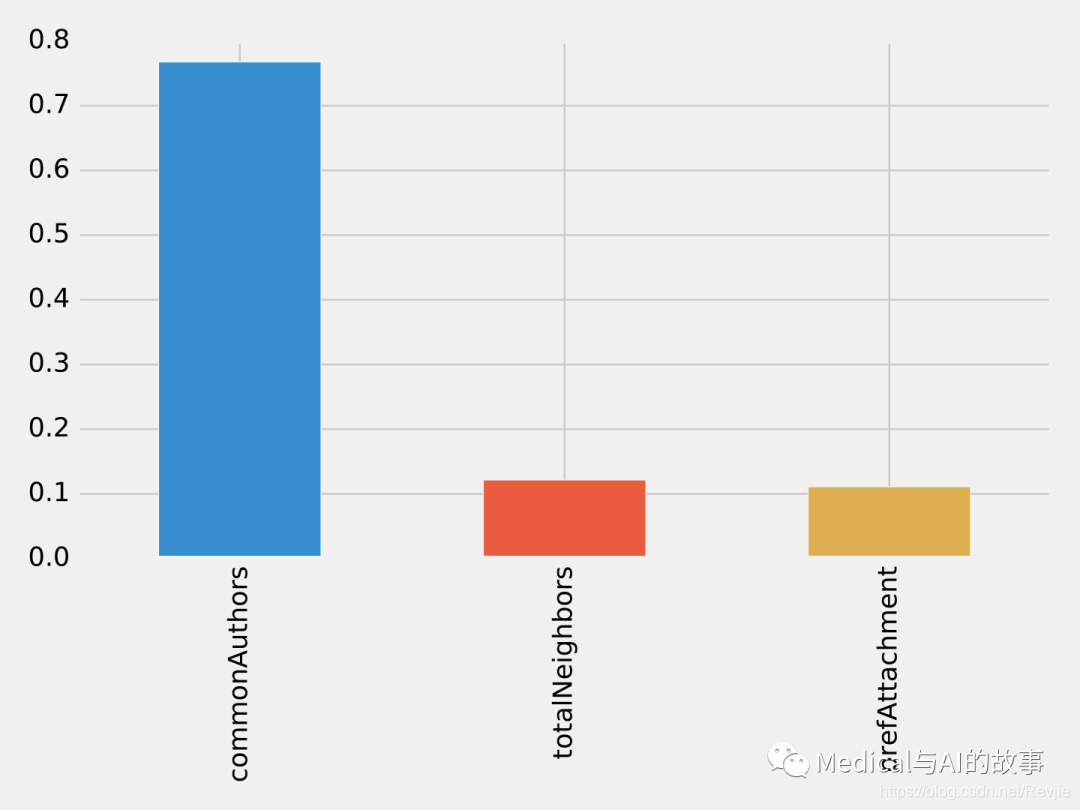
图8-11.特征重要性：图模型
在我们目前使用的三个特征中，commonAuthors在很大程度上是最重要的特征。

为了了解预测模型是如何创建的，我们可以使用spark-tree-plotting库来可视化随机林中的一个决策树。以下代码生成一个GraphViz文件：

from spark_tree_plotting import export_graphviz
dot_string = export_graphviz(rf_model.trees[0],
            featureNames=fields, categoryNames=[], classNames=["True", "False"],
            filled=True, roundedCorners=True, roundLeaves=True)
with open("/tmp/rf.dot", "w") as file:
    file.write(dot_string)

然后，我们可以通过从终端运行以下命令来生成该文件的可视化表示：

dot -Tpdf /tmp/rf.dot -o /tmp/rf.pdf

该命令的输出如图8-12所示。
在这里插入图片描述
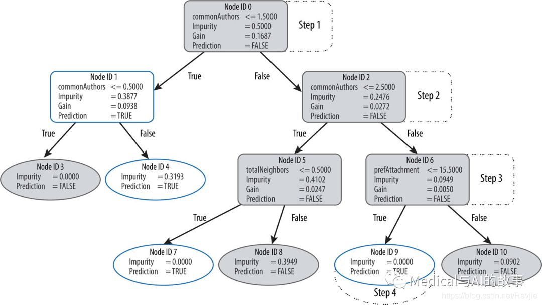
图8-12.可视化决策树

假设我们使用此决策树来预测一对具有以下特征的节点是否链接：

+---------------+----------------+----------------+
| commonAuthors | prefAttachment | totalNeighbors |
+---------------+----------------+----------------+
| 10            | 12             | 5              |
+---------------+----------------+----------------+

我们的随机森林通过几个步骤来建立一个预测：

我们从Node ID 0开始，这里有超过1.5个commonAuthors，所以我们沿着False分支向下到Node ID 2。
我们这里有超过2.5个commonAuthors，所以我们遵循False分支到Node ID 6。
我们的prefAttachment得分低于15.5分，这将我们带到Node ID 9。
Node ID 9是这个决策树中的一个叶节点，这意味着我们不需要再检查任何条件。这个节点上的Pridiction(预测值，比如是True)就是决策树的预测。
最后，随机森林根据这些决策树的集合对所预测的项目进行评估，并根据最可能的结果进行预测。
现在让我们看看添加更多的图特征。

ifeng0310

关注

0
点赞
踩
0

收藏

觉得还不错? 一键收藏
0
评论
《图算法》第八章用图算法增强机器学习-3

对图算法有兴趣的朋友可以关注微信公众号：《 Medical与AI的故事》原文链接：《图算法》第八章-3 用图算法增强机器学习如何评估结果现在让我们根据测试集评估我们的模型。尽管有几种方法可以评估模型的性能，但大多数方法都是根据一些基线预测指标得出的，如表8-1所示：表8-1.预测指标其中，对于TP，FN，FP，TN的解释如下：对于二元分类，根据实际值和预测值的关系，共有四种分类...
复制链接

扫一扫