机器学习升级版第七期——第二课（概率论与贝叶斯先验）

         本总结仅为防止遗忘而作 

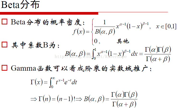
                               常见的分布有

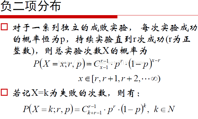
                        关于具体分布的理论部分在此不做过多阐述，可自行查阅资料。其中负二项分布

                        下面给出生活中具体的例子

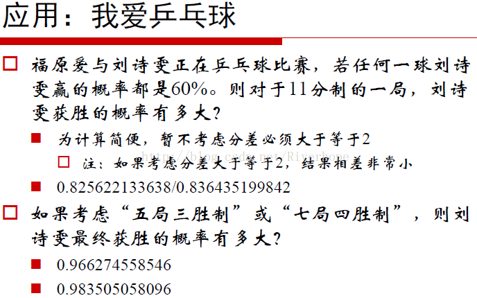
对于上面的例子，若11分制，刘诗雯若获胜那么最后一球肯定是刘诗雯赢的，则对于公式

x=11,r=6,最后一球为刘诗雯赢的，那么前十球中刘诗雯赢5球，即有上面的公式。

下面附上python运行的代码：

import numpy as np
from scipy import special
if __name__ =='__main__':
    method='strict'

    #暴力模拟
    if method =='simulation':
        p = 0.6
        a,b,c = 0,0,0
        t,T = 0,1000000
        while t < T:
            a = b = 0
            while (a <= 11) and (b <= 11):
                if np.random.uniform()<p:
                    a += 1
                else:
                    b += 1
            if a>b:
                c += 1
            t += 1
        print(float(c)/float(T))

    #直接计算
    elif method == 'simple':
        answer = 0
        p = 0.6
        N = 11
        for x in np.arange(N):   #x为对手得分
            answer += special.comb(N+x-1,x)*((1-p)**x)*(p**N)  #scipy.special.comb(N, k)   二项分布
        print(answer)                                         #The number of combinations of N things taken k at a time.
    #严格计算
    else:
        answer = 0
        p = 0.6
        N = 11
        for x in np.arange(N-1):  #x为对手得分 11：9  11:8 11:7 ...
            answer += special.comb(N+x-1,x)*((1-p)**x)*(p**N)
        print(answer)
        p10 = special.comb(2*(N-1),N-1)*((1-p)*p)**(N-1)   # 10:10的概率
        t = 0
        for n in np.arange(100):
            t += (2*p*(1-p))**n*p*p
        answer += p10*t
        print(answer)

==================================================================

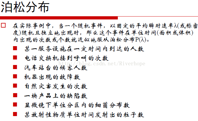
接着生活中现象对应的常见分布：

泊松分布

====================================================================================================

Beta 分布与gamma函数有关，Beta 分布的期望为α/(α+β）

====================================================================================

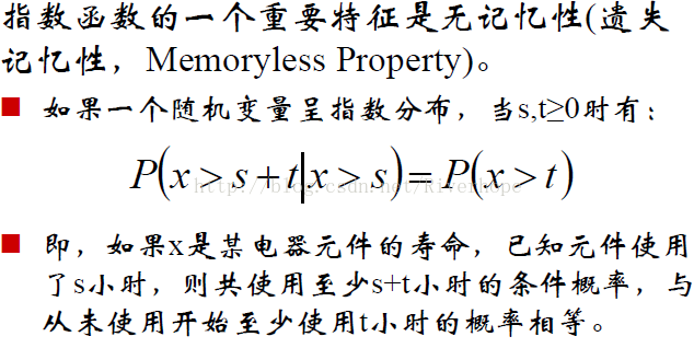
另一个重要的概念

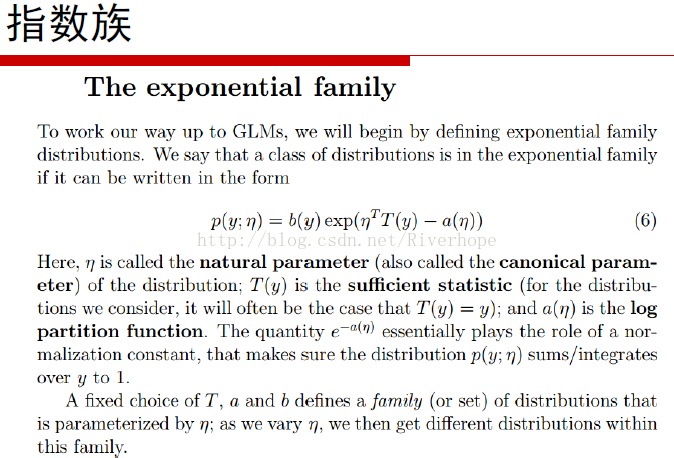
从标题上看，是“指数分布族(exponential family)”，不是“指数分布(exponential distribution)”，这是两个不同的概念。在概率论和统计学中，它是一些有着特殊形式的概率分布的集合，包括许多常用的分布，如normal分布、exponential distribution、bernouli、poission、gamma分布、beta分布等等。指数分布族为很多重要而常用的概率分布提供了统一框架，这种一般性有助于表达的方便和从更大的宏观尺度上理解这些分布.

bernouli分布可以写为：

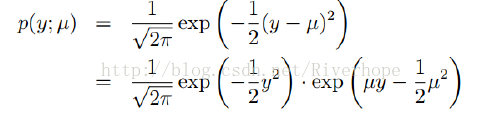
Gaussian分布也属于指数族分布可写为：

=====================================================================

Pearson相关系数：

附上python代码

import numpy as np
from scipy import stats
import matplotlib as mpl
import matplotlib.pyplot as plt
import warnings

mpl.rcParams['axes.unicode_minus'] = False
mpl.rcParams['font.sans-serif'] = 'SimHei'


def calc_pearson(x, y):
    std1 = np.std(x)                               #标准差
    # np.sqrt(np.mean(x**2) - np.mean(x)**2)
    std2 = np.std(y)
    cov = np.cov(x, y, bias=True)[0,1]
    print(np.cov(x,y))
    return cov / (std1 * std2)         # ρ


def intro():
    N = 10
    x = np.random.rand(N)
    y = 2 * x + np.random.randn(N) * 0.1
    print(x)
    print(y)
    print('系统计算：', stats.pearsonr(x, y)[0])         #r是相关系数，取值[-1,1] 表示线性相关程度
    # print(0.0005[0])
    print('手动计算：', calc_pearson(x, y))


def rotate(x, y, theta=45):
    data = np.vstack((x, y))   #vstack   vertical stack ，hstack horizon stack
    print (data)
    mu = np.mean(data, axis=1)
    mu = mu.reshape((-1, 1))
    print('mu=',mu)
    data -= mu
    print ('data-mu=',data)
    theta *= (np.pi / 180)
    c = np.cos(theta)
    s = np.sin(theta)
    m = np.array((c, -s), (s, c))
    print('m=',m)
    return np.dot(m,data) + mu


def pearson(x, y, tip):
    clrs = list('rgbmycrgbmycrgbmycrgbmyc')
    plt.figure(figsize=(10, 8), facecolor='w')
    for i, theta in enumerate(np.linspace(0, 90, 6)):
        xr, yr = rotate(x, y, theta)
        p = stats.pearsonr(xr, yr)[0]
        print (calc_pearson(xr, yr))
        print('旋转角度：', theta, 'Pearson相关系数：', p)
        str = '相关系数：%.3f' % p
        plt.scatter(xr, yr, s=40, alpha=0.9, linewidths=0.5, c=clrs[i], marker='o', label=str)
    plt.legend(loc='upper left', shadow=True)
    plt.xlabel('X')
    plt.ylabel('Y')
    plt.title('Pearson相关系数与数据分布：%s' % tip, fontsize=18)
    plt.grid(b=True)
    plt.show()


if __name__ == '__main__':
    # warnings.filterwarnings(action='ignore', category=RuntimeWarning)
    np.random.seed(0)

    intro()

    N = 1000
    # tip = '一次函数关系'
    # x = np.random.rand(N)
    # y = np.zeros(N) + np.random.randn(N)*0.001
    #
    tip = u'二次函数关系'
    x = np.random.rand(N)
    y = x ** 2 + np.random.randn(N)*0.002
    #
    # tip = u'正切关系'
    # x = np.random.rand(N) * 1.4
    # y = np.tan(x)
    #
    # tip = u'二次函数关系'
    # x = np.linspace(-1, 1, 101)
    # y = x ** 2
    #
    # tip = u'椭圆'
    # x, y = np.random.rand(2, N) * 60 - 30
    # y /= 5
    # idx = (x**2 / 900 + y**2 / 36 < 1)
    # x = x[idx]
    # y = y[idx]

    pearson(x, y, tip)

生成图像为：

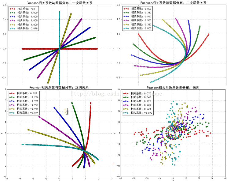
在二次函数图像中可以看出红色线的相关系数为0，但其是具有相关性的，原因为Pearson系数在求取的过程中正负相互抵消导致为0，所以有的时候我们不用Pearson系数进行检验。

======================================================================

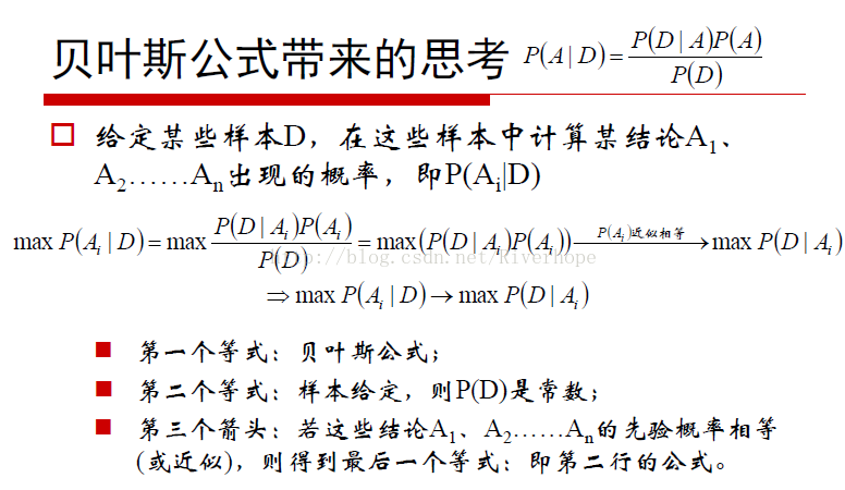
maxP（AlD）在给定样本的情况下，算出A结论的概率取最大，即本来我们是算哪一个结论发生概率最大，那么这个结论是最有可能的，但在日常生活中会反着做maxP（DlA）就是当样本给定时，我们先看发生的概率是多少，然后哪一个结论能够使得我们这个样本发生的概率最大我们就认为那个结论是最容易发生的。（这块有点绕=.=）,一句话就是我们想从数据找原因，其实我们是从原因看数据

最大似然估计：

对于似然函数具体求法不做阐述