高光谱分类

高光谱分类

• 高光谱遥感能够通过成像光谱仪在可见光、近红外、短波
  红外、中红外等电磁波谱范围获取近似连续的光谱曲线，
  将表征地物几何位置关系的空间信息与表征地物属性特征
  的光谱信息有机地融合在了一起，使得提取地物的细节信
  息成为可能。
• 再model中引入注意力机制

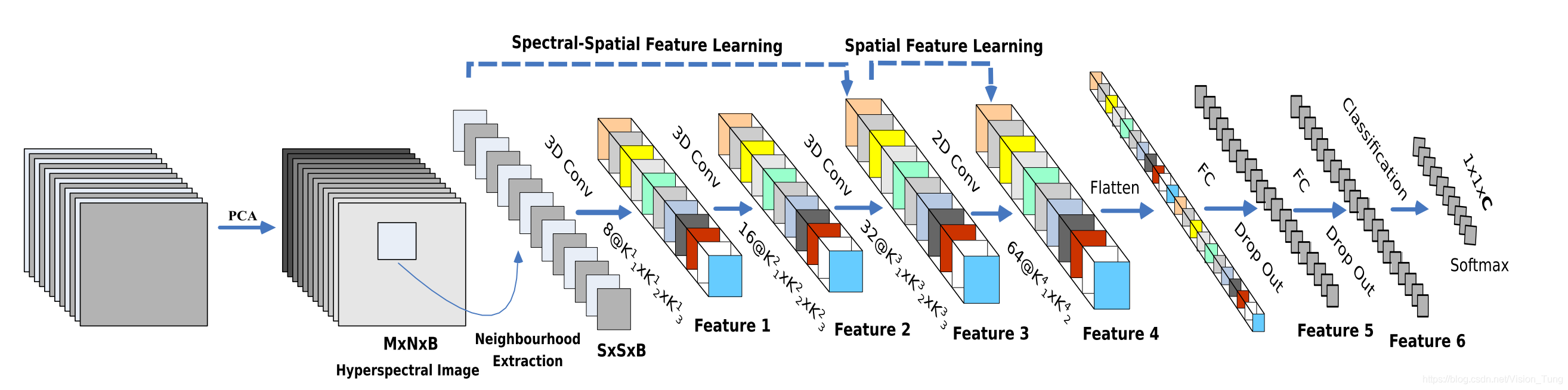
Hybrid-Spectral-Net for Hyperspectral Image Classification.

https://github.com/gokriznastic/HybridSN

 

•  HybridSN是频谱空间3D-CNN，然后是空间2D-CNN。 3D-CNN有助于从一堆光谱带中进行联合空间光谱特征表示。 在3D-CNN之上的2D-CNN进一步学习了更多抽象级别的空间表示。
• Model
  

 colab 代码

https://colab.research.google.com/drive/1aZIZ284KfJUAhUNo1-hSuKW-Eo1QN5Te

 

#库文件
import numpy as np
import matplotlib.pyplot as plt
import scipy.io as sio
from sklearn.decomposition import PCA
from sklearn.model_selection import train_test_split
from sklearn.metrics import confusion_matrix, accuracy_score, classification_report, cohen_kappa_score
import spectral
import torch
import torchvision
import torch.nn as nn
import torch.nn.functional as F
import torch.optim as optim

 Model（已加入注意力机制）

#model

class_num = 16

class HybridSN(nn.Module):
  def __init__(self):
    super(HybridSN,self).__init__()
    self.conv3d1 = nn.Conv3d(1,8,kernel_size=(7,3,3),stride=1,padding=0)
    self.bn1 = nn.BatchNorm3d(8)
    self.conv3d2 = nn.Conv3d(8,16,kernel_size=(5,3,3),stride=1,padding=0)

    self.bn2 = nn.BatchNorm3d(16)
    self.conv3d3 = nn.Conv3d(16,32,kernel_size=(3,3,3),stride=1,padding=0)
    self.bn3 = nn.BatchNorm3d(32)
    self.conv2d4 = nn.Conv2d(576,64,kernel_size=(3,3),stride=1,padding=0)
    self.conv_atetetion=nn.Conv2d(576, 576, kernel_size=(1,1), stride=1, padding=0)
    self.bn4 = nn.BatchNorm2d(64)
    self.softmax=nn.Softmax(dim=1)

    self.fc1 = nn.Linear(18496,8496)
    self.fc2 = nn.Linear(8496,1024)
    self.fc3 = nn.Linear(1024,1024)
    self.fc4 = nn.Linear(1024,256)
    self.fc5 = nn.Linear(256,128)
    self.fc6 = nn.Linear(128,16)
    self.dropout = nn.Dropout(0.4)


  def attention(self, x):
    b, c, h, w = x.size()
    x_phi = self.conv_atetetion(x).view(b, c, -1)
    x_theta = self.conv_atetetion(x).view(b, c, -1).permute(0, 2, 1).contiguous()
    x_g = self.conv_atetetion(x).view(b, c, -1).permute(0, 2, 1).contiguous()
    mul_theta_phi = torch.matmul(x_theta, x_phi)
    mul_theta_phi = self.softmax(mul_theta_phi)
    mul_theta_phi_g = torch.matmul(mul_theta_phi, x_g)
    mul_theta_phi_g = mul_theta_phi_g.permute(0,2,1).contiguous().view(b, c, h, w)
    mask = self.conv_atetetion(mul_theta_phi_g)
    out = mask + x
    return out

  def forward(self,x):
    out = F.relu(self.bn1(self.conv3d1(x)))
    out = F.relu(self.bn2(self.conv3d2(out)))
    out = F.relu(self.bn3(self.conv3d3(out)))
    out = self.attention(out.reshape(out.shape[0],-1,19,19))
    out = F.relu(self.bn4(self.conv2d4(out)))
    
    out = out.reshape(out.shape[0],-1)
    out = F.relu(self.dropout(self.fc1(out)))
    out = F.relu(self.dropout(self.fc2(out)))
    out = F.relu(self.dropout(self.fc3(out)))
    out = F.relu(self.dropout(self.fc4(out)))
    out = F.relu(self.dropout(self.fc5(out)))
    out = self.fc6(out)
    return out
#随机输入，测试网络结构是否通
x = torch.randn(1, 1, 30, 25, 25)
net = HybridSN()
y = net(x)
print(y.shape)

# 对高光谱数据 X 应用 PCA 变换

def applyPCA(X, numComponents):
    newX = np.reshape(X, (-1, X.shape[2]))
    pca = PCA(n_components=numComponents, whiten=True)
    newX = pca.fit_transform(newX)
    newX = np.reshape(newX, (X.shape[0], X.shape[1], numComponents))
    return newX


# 对单个像素周围提取 patch 时，边缘像素就无法取了，因此，给这部分像素进行 padding 操作
def padWithZeros(X, margin=2):
    newX = np.zeros((X.shape[0] + 2 * margin, X.shape[1] + 2* margin, X.shape[2]))
    x_offset = margin
    y_offset = margin
    newX[x_offset:X.shape[0] + x_offset, y_offset:X.shape[1] + y_offset, :] = X
    return newX

# 在每个像素周围提取 patch ，然后创建成符合 keras 处理的格式
def createImageCubes(X, y, windowSize=5, removeZeroLabels = True):
    # 给 X 做 padding
    margin = int((windowSize - 1) / 2)
    zeroPaddedX = padWithZeros(X, margin=margin)
    # split patches
    patchesData = np.zeros((X.shape[0] * X.shape[1], windowSize, windowSize, X.shape[2]))
    patchesLabels = np.zeros((X.shape[0] * X.shape[1]))
    patchIndex = 0
    for r in range(margin, zeroPaddedX.shape[0] - margin):
        for c in range(margin, zeroPaddedX.shape[1] - margin):
            patch = zeroPaddedX[r - margin:r + margin + 1, c - margin:c + margin + 1]   
            patchesData[patchIndex, :, :, :] = patch
            patchesLabels[patchIndex] = y[r-margin, c-margin]
            patchIndex = patchIndex + 1
    if removeZeroLabels:
        patchesData = patchesData[patchesLabels>0,:,:,:]
        patchesLabels = patchesLabels[patchesLabels>0]
        patchesLabels -= 1
    return patchesData, patchesLabels

def splitTrainTestSet(X, y, testRatio, randomState=345):
    X_train, X_test, y_train, y_test = train_test_split(X, y, test_size=testRatio, random_state=randomState, stratify=y)
    return X_train, X_test, y_train, y_test

# 地物类别
class_num = 16
X = sio.loadmat('Indian_pines_corrected.mat')['indian_pines_corrected']
y = sio.loadmat('Indian_pines_gt.mat')['indian_pines_gt']

# 用于测试样本的比例
test_ratio = 0.90
    # 每个像素周围提取 patch 的尺寸
patch_size = 25
# 使用 PCA 降维，得到主成分的数量
pca_components = 30

print('Hyperspectral data shape: ', X.shape)
print('Label shape: ', y.shape)

print('\n... ... PCA tranformation ... ...')
X_pca = applyPCA(X, numComponents=pca_components)
print('Data shape after PCA: ', X_pca.shape)

print('\n... ... create data cubes ... ...')
X_pca, y = createImageCubes(X_pca, y, windowSize=patch_size)
print('Data cube X shape: ', X_pca.shape)
print('Data cube y shape: ', y.shape)

print('\n... ... create train & test data ... ...')
Xtrain, Xtest, ytrain, ytest = splitTrainTestSet(X_pca, y, test_ratio)
print('Xtrain shape: ', Xtrain.shape)
print('Xtest  shape: ', Xtest.shape)

# 改变 Xtrain, Ytrain 的形状，以符合 keras 的要求
Xtrain = Xtrain.reshape(-1, patch_size, patch_size, pca_components, 1)
Xtest  = Xtest.reshape(-1, patch_size, patch_size, pca_components, 1)
print('before transpose: Xtrain shape: ', Xtrain.shape) 
print('before transpose: Xtest  shape: ', Xtest.shape) 

# 为了适应 pytorch 结构，数据要做 transpose
Xtrain = Xtrain.transpose(0, 4, 3, 1, 2)
Xtest  = Xtest.transpose(0, 4, 3, 1, 2)
print('after transpose: Xtrain shape: ', Xtrain.shape) 
print('after transpose: Xtest  shape: ', Xtest.shape) 


""" Training dataset"""
class TrainDS(torch.utils.data.Dataset): 
    def __init__(self):
        self.len = Xtrain.shape[0]
        self.x_data = torch.FloatTensor(Xtrain)
        self.y_data = torch.LongTensor(ytrain)        
    def __getitem__(self, index):
        # 根据索引返回数据和对应的标签
        return self.x_data[index], self.y_data[index]
    def __len__(self): 
        # 返回文件数据的数目
        return self.len

""" Testing dataset"""
class TestDS(torch.utils.data.Dataset): 
    def __init__(self):
        self.len = Xtest.shape[0]
        self.x_data = torch.FloatTensor(Xtest)
        self.y_data = torch.LongTensor(ytest)
    def __getitem__(self, index):
        # 根据索引返回数据和对应的标签
        return self.x_data[index], self.y_data[index]
    def __len__(self): 
        # 返回文件数据的数目
        return self.len

# 创建 trainloader 和 testloader
trainset = TrainDS()
testset  = TestDS()
train_loader = torch.utils.data.DataLoader(dataset=trainset, batch_size=128, shuffle=True, num_workers=2)
test_loader  = torch.utils.data.DataLoader(dataset=testset,  batch_size=128, shuffle=False, num_workers=2)

# 使用GPU训练，可以在菜单 "代码执行工具" -> "更改运行时类型" 里进行设置
device = torch.device("cuda:0" if torch.cuda.is_available() else "cpu")

# 网络放到GPU上
net = HybridSN().to(device)
criterion = nn.CrossEntropyLoss()
optimizer = optim.Adam(net.parameters(), lr=0.001)

# 开始训练
total_loss = 0
for epoch in range(100):
    for i, (inputs, labels) in enumerate(train_loader):
        inputs = inputs.to(device)
        labels = labels.to(device)
        # 优化器梯度归零
        optimizer.zero_grad()
        # 正向传播 +　反向传播 + 优化 
        outputs = net(inputs)
        loss = criterion(outputs, labels)
        loss.backward()
        optimizer.step()
        total_loss += loss.item()
    print('[Epoch: %d]   [loss avg: %.4f]   [current loss: %.4f]' %(epoch + 1, total_loss/(epoch+1), loss.item()))

print('Finished Training')

count = 0
# 模型测试
for inputs, _ in test_loader:
    inputs = inputs.to(device)
    outputs = net(inputs)
    outputs = np.argmax(outputs.detach().cpu().numpy(), axis=1)
    if count == 0:
        y_pred_test =  outputs
        count = 1
    else:
        y_pred_test = np.concatenate( (y_pred_test, outputs) )

# 生成分类报告
classification = classification_report(ytest, y_pred_test, digits=4)
print(classification)

from operator import truediv

def AA_andEachClassAccuracy(confusion_matrix):
    counter = confusion_matrix.shape[0]
    list_diag = np.diag(confusion_matrix)
    list_raw_sum = np.sum(confusion_matrix, axis=1)
    each_acc = np.nan_to_num(truediv(list_diag, list_raw_sum))
    average_acc = np.mean(each_acc)
    return each_acc, average_acc


def reports (test_loader, y_test, name):
    count = 0
    # 模型测试
    for inputs, _ in test_loader:
        inputs = inputs.to(device)
        outputs = net(inputs)
        outputs = np.argmax(outputs.detach().cpu().numpy(), axis=1)
        if count == 0:
            y_pred =  outputs
            count = 1
        else:
            y_pred = np.concatenate( (y_pred, outputs) )

    if name == 'IP':
        target_names = ['Alfalfa', 'Corn-notill', 'Corn-mintill', 'Corn'
                        ,'Grass-pasture', 'Grass-trees', 'Grass-pasture-mowed', 
                        'Hay-windrowed', 'Oats', 'Soybean-notill', 'Soybean-mintill',
                        'Soybean-clean', 'Wheat', 'Woods', 'Buildings-Grass-Trees-Drives',
                        'Stone-Steel-Towers']
    elif name == 'SA':
        target_names = ['Brocoli_green_weeds_1','Brocoli_green_weeds_2','Fallow','Fallow_rough_plow','Fallow_smooth',
                        'Stubble','Celery','Grapes_untrained','Soil_vinyard_develop','Corn_senesced_green_weeds',
                        'Lettuce_romaine_4wk','Lettuce_romaine_5wk','Lettuce_romaine_6wk','Lettuce_romaine_7wk',
                        'Vinyard_untrained','Vinyard_vertical_trellis']
    elif name == 'PU':
        target_names = ['Asphalt','Meadows','Gravel','Trees', 'Painted metal sheets','Bare Soil','Bitumen',
                        'Self-Blocking Bricks','Shadows']
    
    classification = classification_report(y_test, y_pred, target_names=target_names)
    oa = accuracy_score(y_test, y_pred)
    confusion = confusion_matrix(y_test, y_pred)
    each_acc, aa = AA_andEachClassAccuracy(confusion)
    kappa = cohen_kappa_score(y_test, y_pred)
    
    return classification, confusion, oa*100, each_acc*100, aa*100, kappa*100

classification, confusion, oa, each_acc, aa, kappa = reports(test_loader, ytest, 'IP')
classification = str(classification)
confusion = str(confusion)
file_name = "classification_report.txt"

with open(file_name, 'w') as x_file:
    x_file.write('\n')
    x_file.write('{} Kappa accuracy (%)'.format(kappa))
    x_file.write('\n')
    x_file.write('{} Overall accuracy (%)'.format(oa))
    x_file.write('\n')
    x_file.write('{} Average accuracy (%)'.format(aa))
    x_file.write('\n')
    x_file.write('\n')
    x_file.write('{}'.format(classification))
    x_file.write('\n')
    x_file.write('{}'.format(confusion))

# load the original image
X = sio.loadmat('Indian_pines_corrected.mat')['indian_pines_corrected']
y = sio.loadmat('Indian_pines_gt.mat')['indian_pines_gt']

height = y.shape[0]
width = y.shape[1]

X = applyPCA(X, numComponents= pca_components)
X = padWithZeros(X, patch_size//2)

# 逐像素预测类别
outputs = np.zeros((height,width))
for i in range(height):
    for j in range(width):
        if int(y[i,j]) == 0:
            continue
        else :
            image_patch = X[i:i+patch_size, j:j+patch_size, :]
            image_patch = image_patch.reshape(1,image_patch.shape[0],image_patch.shape[1], image_patch.shape[2], 1)
            X_test_image = torch.FloatTensor(image_patch.transpose(0, 4, 3, 1, 2)).to(device)                                   
            prediction = net(X_test_image)
            prediction = np.argmax(prediction.detach().cpu().numpy(), axis=1)
            outputs[i][j] = prediction+1
    if i % 20 == 0:
        print('... ... row ', i, ' handling ... ...')


predict_image = spectral.imshow(classes = outputs.astype(int),figsize =(5,5))

 结果