学习常用模型及算法：1.启发式算法（模拟退火和遗传算法）

启发式算法常见的有三种：模拟退火、遗传算法、神经网络

本篇文章主要涉及模拟退火和遗传算法。

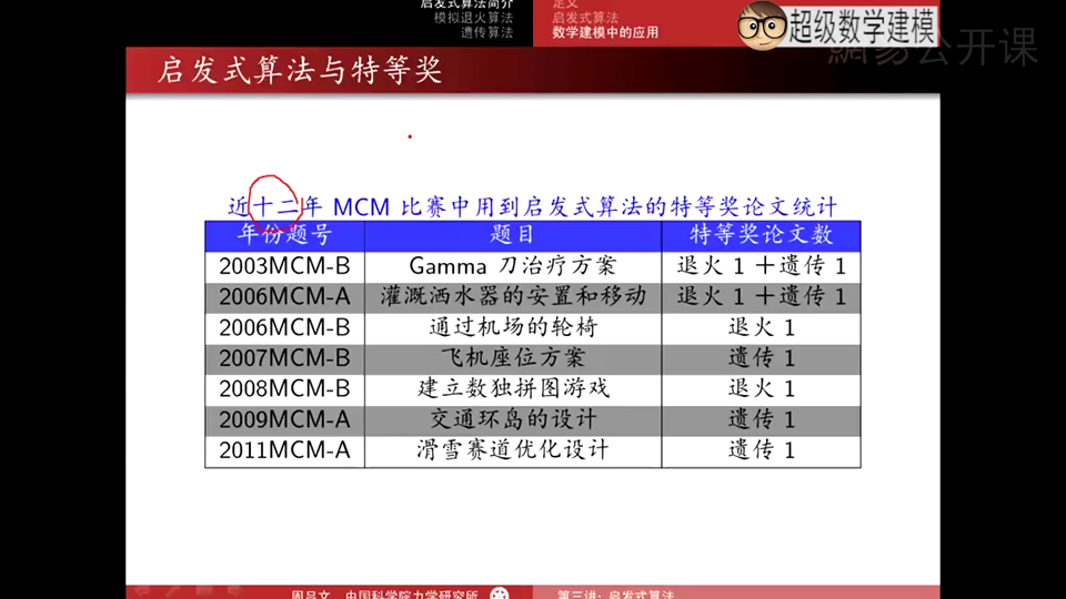
事实证明，即使是老算法也能用的很妙。

 

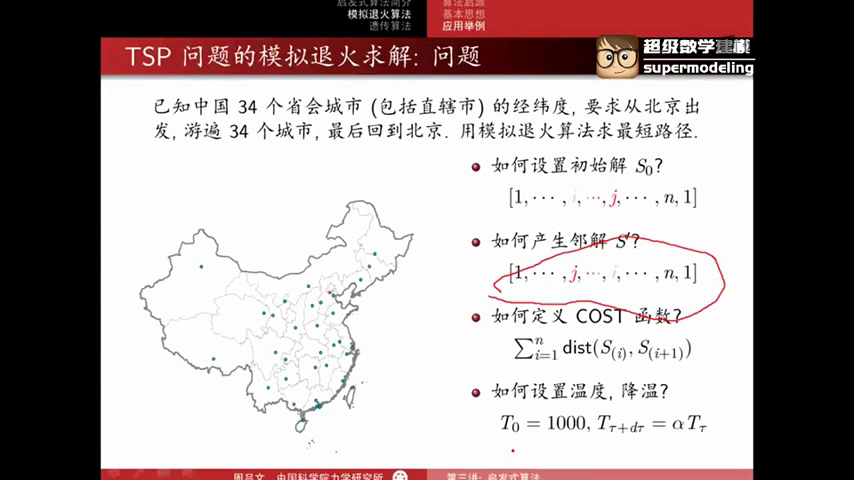
经典问题：旅行商问题(TSP)

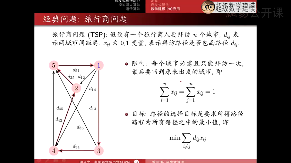
每个城市只有一个箭头指进，一个箭头指出，即入度和出度均为1。

 

模拟退火算法原理

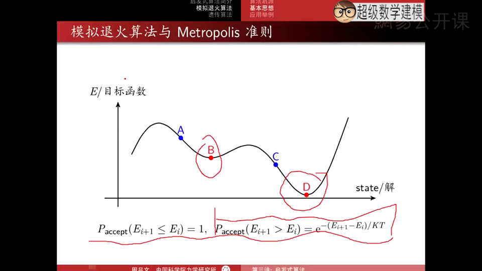
模拟退火算法的好处就在于，如果你设置初始点为A点，会有一定概率跳出B点从而到达D点，而贪心算法不行（除非设置初始点在C点）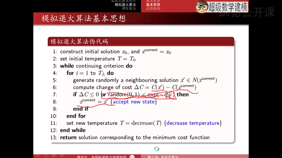

图中or random...即为metropolis准则，也是模拟退火和贪心算法的根本区别。

 

模拟退火算法设计要素

在设计模拟退火算法解决问题中，我们需要注意以下几个要素：

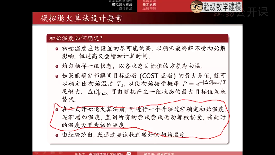
确定初始温度的方法中，多设几个温度，逐渐增加温度是最靠谱的。

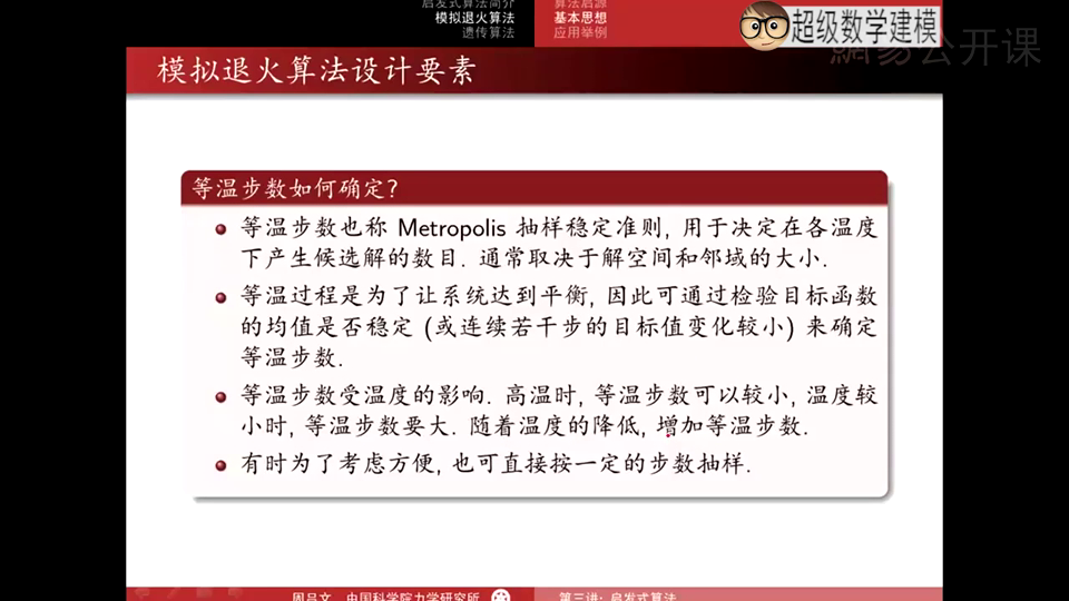
如果解空间非常小，等温步数可能要小一点；如果解空间非常大，等温步数可能要大一点。

虽然等温步数受温度影响，但一般情况下，不论低温和高温时，等温步数都设大一点。

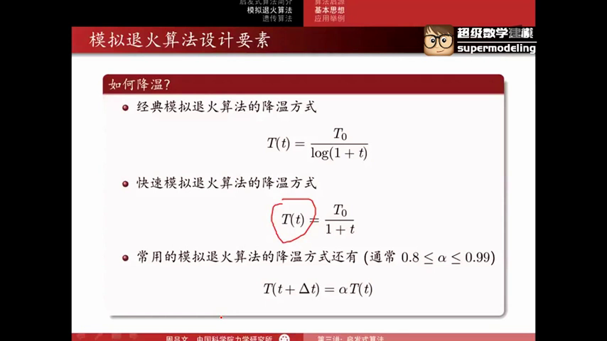
三种降温方式

 

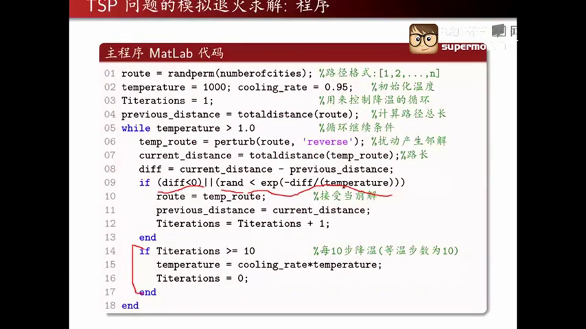
用模糊退火来求解TSP问题

 

代码详解

perturb和totaldistance是自己建立的函数

perturb用来产生邻解，totaldistance求总长。

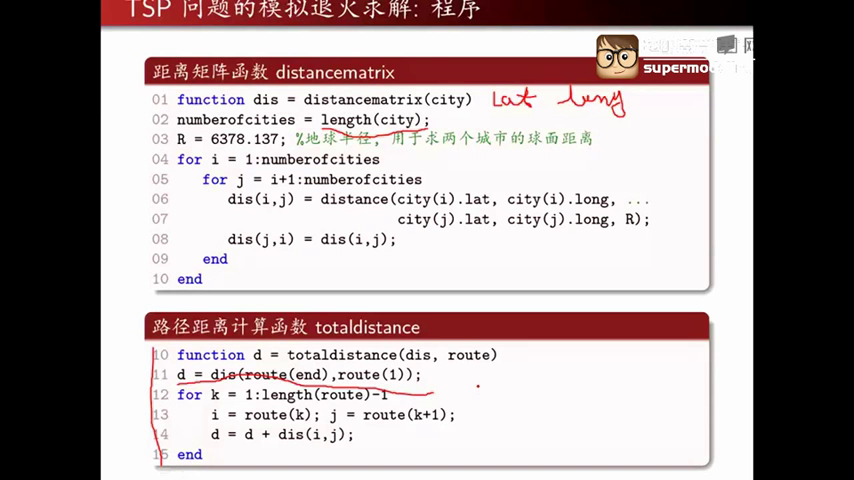
distance函数中，输入两点经纬度和地球半径，即可求出两点间的球面距离。

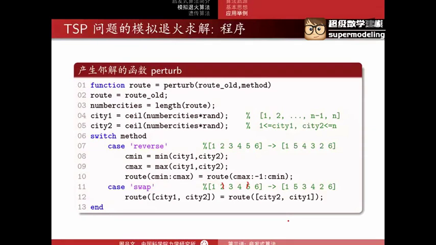
ceil(numbercities*rand)用来产生1到37之间的任意数。

产生邻解的方法有两种，一种是“reverse”，另一种是“swap”。

 

代码实现

main.m

%
% This is the main script to finds a (near) optimal solution to the Traveling
% Salesman Problem (TSP), by setting up a Simulated Annealing (SA) to search 
% for the shortest route (least distance for the salesman to travel to each 
% city exactly once and return to the starting city).
%
% Author: zhou lvwen       Email: zhou.lv.wen@gmail.com
% Release Date: November 12, 2012
%

clear;clc;

load china; % geographic information
plotcities(province, border, city); % draw the map of China

numberofcities = length(city);      % number of cities
% distance matrix: dis(i,j) is the distance between city i and j.
dis = distancematrix(city);   


temperature = 1000;                 % Initialize the temperature.
cooling_rate = 0.94;                % cooling rate
iterations = 1;                     % Initialize the iteration number.

% Initialize random number generator with "seed". 
rand('seed',0);                    

% Initialize the route by generate a sequence of random
route = randperm(numberofcities);
% This is objective function, the total distance for the routes.
previous_distance = totaldistance(route,dis);

% This is a flag used to cool the current temperature after 100 iterations
temperature_iterations = 1;
% This is a flag used to plot the current route after 200 iterations
plot_iterations = 1;

% plot the current route
plotroute(city, route, previous_distance, temperature);

while 1.0 < temperature
    % generate randomly a neighbouring solution
    temp_route = perturb(route,'reverse');
    % compute total distance of the temp_route
    current_distance = totaldistance(temp_route, dis);
    % compute change of distance
    diff = current_distance - previous_distance;
    
    % Metropolis Algorithm
    if (diff < 0) || (rand < exp(-diff/(temperature)))
        route = temp_route;         %accept new route
        previous_distance = current_distance;
        
        % update iterations
        temperature_iterations = temperature_iterations + 1;
        plot_iterations = plot_iterations + 1;
        iterations = iterations + 1;
    end
    
    % reduce the temperature every 100 iterations
    if temperature_iterations >= 100
       temperature = cooling_rate*temperature;
       temperature_iterations = 0;
    end
    
    %  plot the current route every 200 iterations
    if plot_iterations >= 200
       plotroute(city, route, previous_distance,temperature);
       plot_iterations = 0;
    end
end

% plot the final solution
plotroute(city, route, previous_distance,temperature);

distancematrix.m

function dis = distancematrix(city)
% DISTANCEMATRIX
% dis = DISTANCEMATRIX(city) return the distance matrix, dis(i,j) is the 
% distance between city_i and city_j

numberofcities = length(city);
R = 6378.137; % The radius of the Earth
for i = 1:numberofcities
    for j = i+1:numberofcities
        dis(i,j) = distance(city(i).lat, city(i).long, ...
                            city(j).lat, city(j).long, R);
        dis(j,i) = dis(i,j);
    end
end


function d = distance(lat1, long1, lat2, long2, R)
% DISTANCE
% d = DISTANCE(lat1, long1, lat2, long2, R) compute distance between points
% on sphere with radians R.
%
% Latitude/Longitude Distance Calculation:
% http://www.mathforum.com/library/drmath/view/51711.html
 
y1 = lat1/180*pi; x1 = long1/180*pi;
y2 = lat2/180*pi; x2 = long2/180*pi;
dy = y1-y2; dx = x1-x2;
d = 2*R*asin(sqrt(sin(dy/2)^2+sin(dx/2)^2*cos(y1)*cos(y2)));

totaldistance.m

function d = totaldistance(route, dis)
% TOTALDISTANCE
% d = TOTALDISTANCE(route, dis) calculate total distance of a route with
% the distance matrix dis.

d = dis(route(end),route(1)); % closed path
for k = 1:length(route)-1
    i = route(k);
    j = route(k+1);
    d = d + dis(i,j);
end

perturb.m

function route = perturb(route_old, method)
% PERTURB
% route = PERTURB(route_old, method) generate randomly a neighbouring route by
% perturb old route. perturb methods:
%                        ___________            ___________         
%     1. reverse:   [1 2 3 4 5 6 7 8 9] -> [1 2 8 7 6 5 4 3 9]
%                        _         _            _         _
%     2. swap:      [1 2 3 4 5 6 7 8 9] -> [1 2 8 4 5 6 7 3 9]

route = route_old;
numbercities = length(route);
city1 = ceil(numbercities*rand);
city2 = ceil(numbercities*rand);
switch method
    case 'reverse'
        citymin = min(city1,city2);
        citymax = max(city1,city2);
        route(citymin:citymax) = route(citymax:-1:citymin);
    case 'swap'
        route([city1, city2]) = route([city2, city1]);
end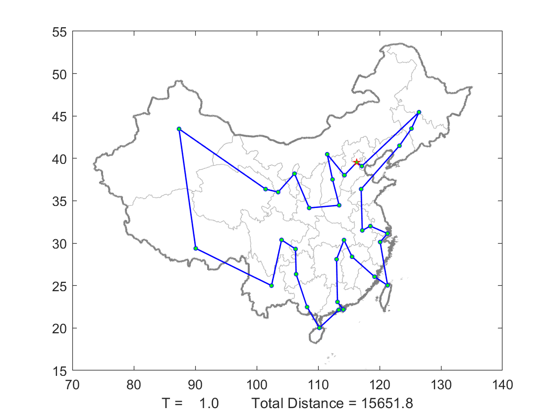

退火算法不一定是最优解，但却是空间和时间花费比较小的算法。

实际上解决TSP问题的最优解可用整数规划求得。

 

遗传算法原理

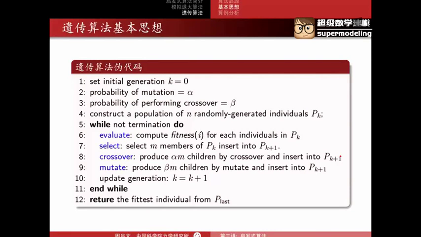
前四行分别为初代、变异概率、杂交概率、含有n个初始解的种群。

在最后一代中选出最优秀的一个。

 

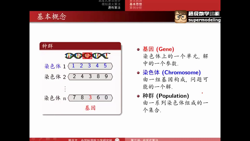
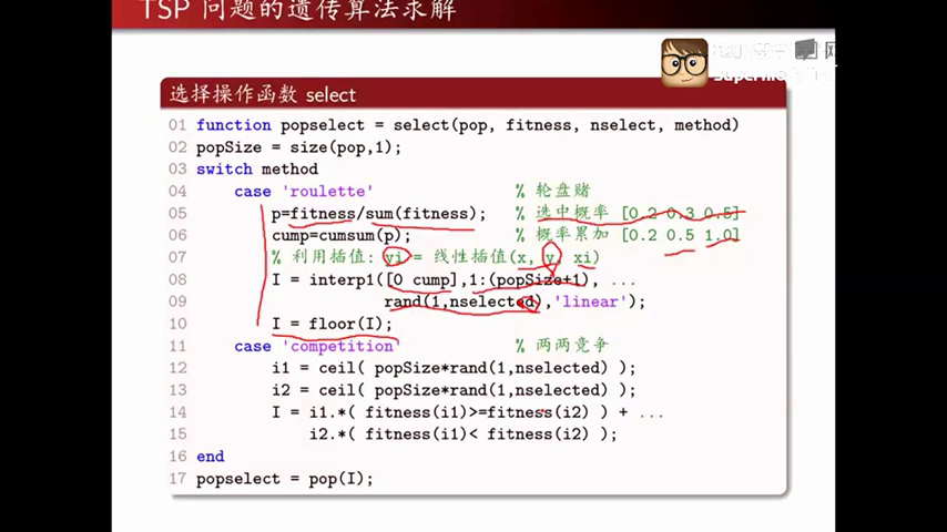
与遗传算法有关的一些概念

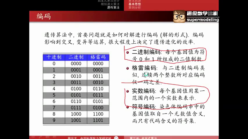
在编码中，实数编码和二进制编码是最常用到的。

排序选择的随机性比较小一些，轮盘赌和两两竞争的随机性比较大一些。

 

用遗传算法来求解TSP问题

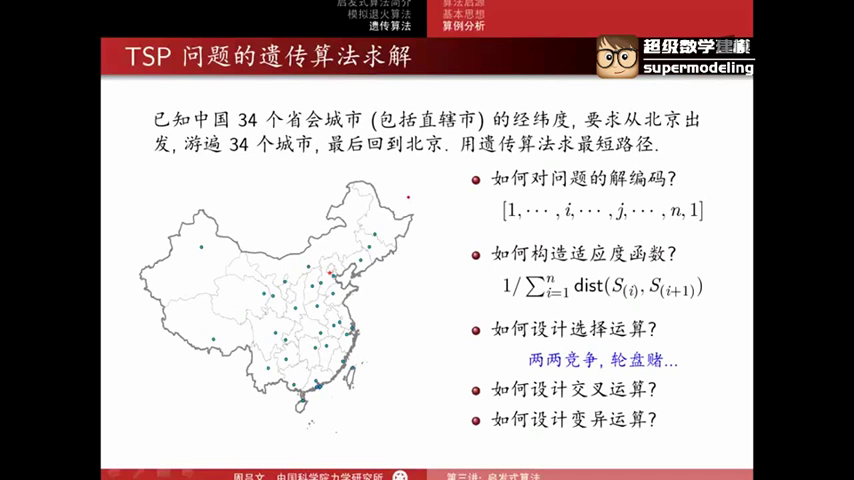
这里为了让适应度函数足够小，取总距离的倒数。

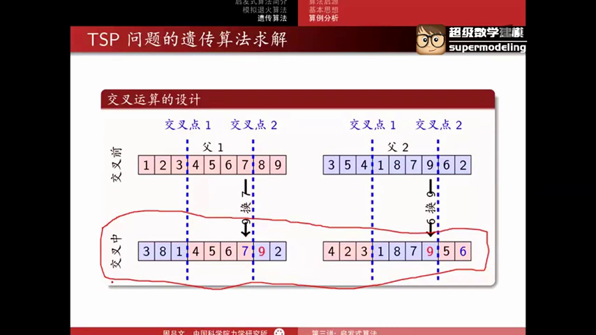
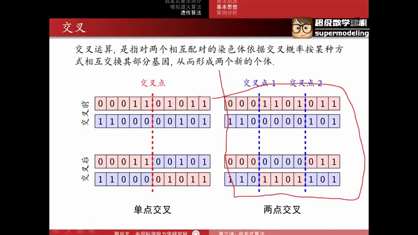
这里的交叉运算和先前的直接交叉有所差别。这和解的特征有所关联。将上面的4传给下面的1以后，下面的1变为4，但另一个原本的4与新的4重复，所以原本的4又变成1。

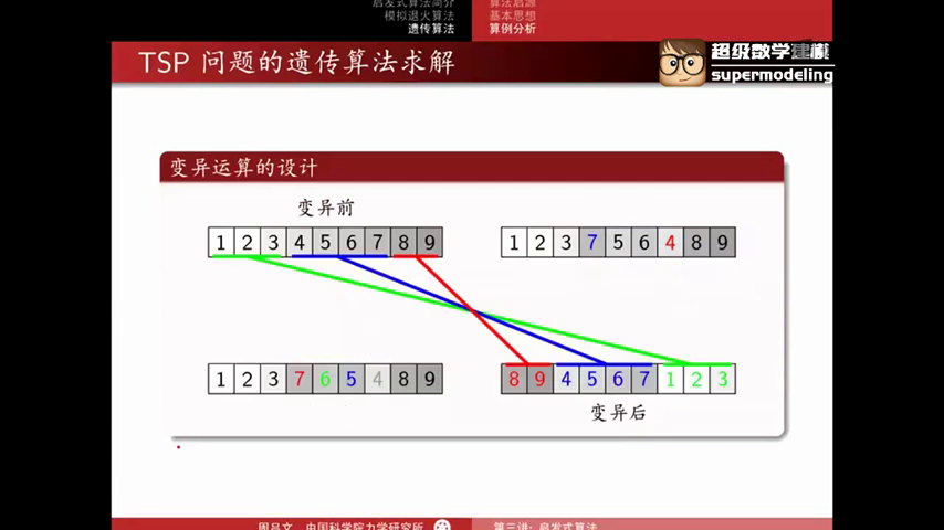
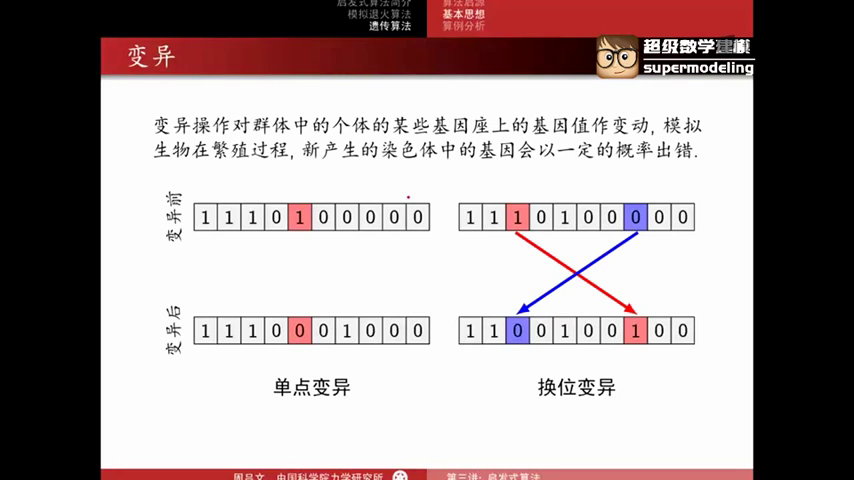
这里的变异和扰动有些类似。

 

代码详解

pop为初始化的种群

select选择  crossover交叉  mutate变异

第14行是为了将最好的解留在种群当中

size(pop, 1)求出pop的行数，即种群的个数

第12行可理解为：在1至popSize的整数之间任意挑选nselect次（可重复）之后组成的数组。

interp1为线性插值函数

I是我们选择的行数，即我们选择了哪些个体。

InsertPoints决定了我们进行交叉操作的起点与终点。

具体交叉方式与前文所述类似。

待交叉结束后，将child1和child2插回children。

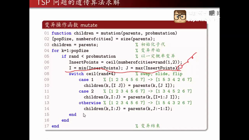
当rand小于probmutation时，发生变异，变异情况有三种，1/4的可能性swap，1/4的可能性slide，1/2的可能性flip。

 

代码实现

main.m

%
% This is the main script to finds a (near) optimal solution to the Traveling
% Salesman Problem (TSP), by setting up a Genetic Algorithm (GA) to search 
% for the shortest route (least distance for the salesman to travel to each 
% city exactly once and return to the starting city).
%
% Author: zhou lvwen       Email: zhou.lv.wen@gmail.com
% Release Date: November 12, 2012
%

clear;clc;

load china;                         % geographic information
plotcities(province, border, city); % draw the map of China

numberofcities = length(city);      % number of cities
% distance matrix: dis(i,j) is the distance between city i and j.
dis = distancematrix(city);   

popSize = 100;                      % population size
max_generation = 1000;              % number of generation
probmutation = 0.16;                % probability of mutation

% Initialize random number generator with "seed". 
rand('seed',103);
% Initialize the pop: start from random routes
pop = zeros(popSize,numberofcities); 
for i=1:popSize
    pop(i,:)=randperm(numberofcities);
end


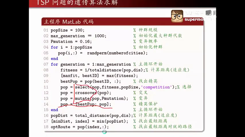
for generation = 1:max_generation   % generations loop
    
    % evaluate: compute fitness(1/totaldistance) for each individuals in pop
    popDist = totaldistance(pop,dis);
    fitness = 1./popDist;
   
    % find the best route & distance
    [mindist, bestID] = min(popDist); 
    bestPop = pop(bestID, :);       % best route
    
    % update best route on figure:
    if mod(generation,10)==0
        plotroute(city, bestPop, mindist, generation)
    end
    
    % select (competition / roulette)
    pop = select(pop, fitness, popSize,'competition');
    
    % crossover
    pop = crossover(pop);
    
    % mutation
    pop = mutation(pop, probmutation);
   
    % save elitism(best path) and put it to next generation without changes
    pop = [bestPop; pop];
end

% return the best route
[mindist, bestID]=min(popDist); 
bestPop = pop(bestID, :);

% plot the final solution
plotroute(city, bestPop, mindist, generation);

select.m

function popselected = select(pop, fitness, nselected, method)
% SELECT
% popselected = SELECT(pop, fitness, nselected, method) select the fittest 
% individuals to survive to the next generation.
%

popSize = size(pop,1);

switch method
    
    case 'roulette'
        p=fitness/sum(fitness); % probabilities of select
        cump=cumsum(p);         % cumulative sum of probabilities
        I = interp1([0 cump],1:(popSize+1),rand(1,nselected),'linear');
        % random numbers from 1:nselected according probabilities
        I = floor(I); 
        
    case 'competition'
        % randomly generated two sets of population
        i1 = ceil( popSize*rand(1,nselected) );
        i2 = ceil( popSize*rand(1,nselected) );
        % compare the fitness and select the fitter
        I = i1.*( fitness(i1)>=fitness(i2) ) + ...
            i2.*( fitness(i1)< fitness(i2) );
        
end

popselected=pop(I,:);

function children = crossover(parents)
% CROSSOVER
% children = CROSSOVER(parents) Replicate the mating process by crossing 
% over randomly selected parents. 
%
% Mapped Crossover (PMX) example:     
%           _                          _                          _
%    [1 2 3|4 5 6 7|8 9]  |-> [4 2 3|1 5 6 7|8 9]  |-> [4 2 3|1 8 6 7|5 9]
%    [3 5 4|1 8 7 6|9 2]  |   [3 5 1|4 8 7 6|9 2]  |   [3 8 1|4 5 7 6|9 2]
%           |             |            |           |              |            
%           V             |            V           |              |  
%    [* 2 3|1 5 6 7|8 9] _|   [4 2 3|1 8 6 7|* 9] _|              V
%    [3 5 *|4 8 7 6|9 2]      [3 * 1|4 5 7 6|9 2]           ... ... ...
%

[popSize, numberofcities] = size(parents);    
children = parents; % childrens

for i = 1:2:popSize % pairs counting
    parent1 = parents(i+0,:);  child1 = parent1;
    parent2 = parents(i+1,:);  child2 = parent2;
    % chose two random points of cross-section
    InsertPoints = sort(ceil(numberofcities*rand(1,2)));
    for j = InsertPoints(1):InsertPoints(2)
        if parent1(j)~=parent2(j)
            child1(child1==parent2(j)) = child1(j);
            child1(j) = parent2(j);
            
            child2(child2==parent1(j)) = child2(j);
            child2(j) = parent1(j);
        end
    end
    % two childrens:
    children(i+0,:)=child1;     children(i+1,:)=child2;
end

mutation.m

function children = mutation(parents, probmutation)
% MUTATION
% children = MUTATION(parents, probmutation) Replicate mutation in the 
% population by  selecting an individual with probability probmutation
%     
% swap:    _         _    slide:    _ _________    flip:     ---------->
%     [1 2|3 4 5 6 7 8|9]      [1 2|3 4 5 6 7 8|9]      [1 2|3 4 5 6 7 8|9] 
%                                   _________ _              <----------
%     [1 2|8 4 5 6 7 3|9]      [1 2|4 5 6 7 8 3|9]      [1 2|8 7 6 5 4 3|9]
%

[popSize, numberofcities] = size(parents);
children = parents;
for k=1:popSize
    if rand < probmutation
       InsertPoints = ceil(numberofcities*rand(1,2));
       I = min(InsertPoints);  J = max(InsertPoints);
       switch ceil(rand*6)
           case 1    % swap
             children(k,[I J]) = parents(k,[J I]);
           case 2    % slide
             children(k,[I:J]) = parents(k,[I+1:J I]);
           otherwise % flip
             children(k,[I:J]) = parents(k,[J:-1:I]);
       end
    end
end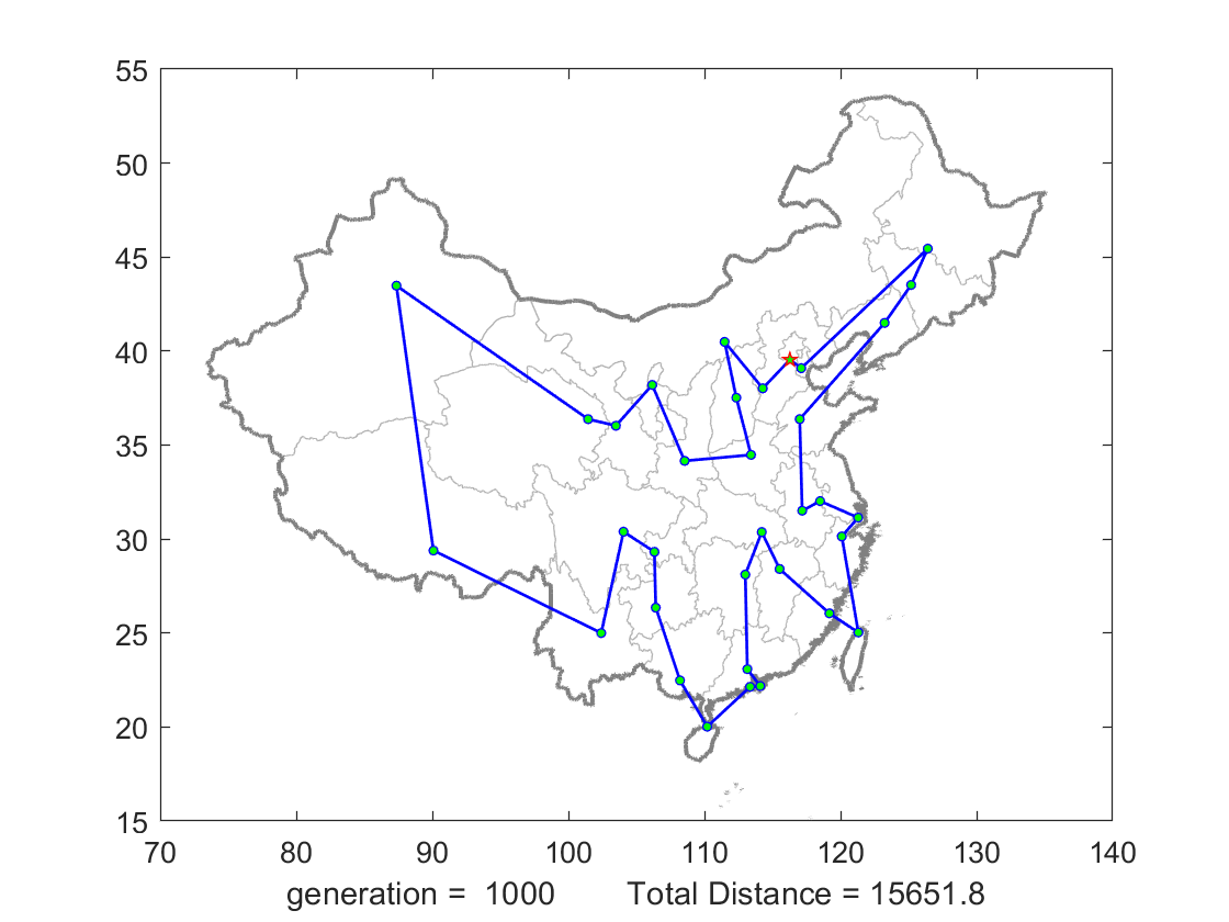

与模拟退火算法所获得的答案是一致的。（应该只是巧合……？）

模拟退火算法和遗传算法在本质上都是不断调整，寻求最优解的过程。

重点：多看伪代码，加深理解。