sklearn分类场景案例01

import numpy as np
import matplotlib.pyplot as plt
from sklearn import datasets
from sklearn.model_selection import train_test_split
from sklearn.preprocessing import StandardScaler
from sklearn.svm import SVC
from sklearn.metrics import classification_report, confusion_matrix, accuracy_score
from sklearn.pipeline import make_pipeline

# 1. 加载数据
iris = datasets.load_iris()
X = iris.data[:, :2]  # 只取前两个特征便于可视化
y = iris.target

# 2. 划分训练集和测试集
X_train, X_test, y_train, y_test = train_test_split(
    X, y, test_size=0.3, random_state=42
)

# 3. 创建模型管道（预处理+分类器）
model = make_pipeline(
    StandardScaler(),  # 特征标准化
    SVC(kernel='rbf', gamma='auto')  # 使用SVM分类器
)

# 4. 训练模型
model.fit(X_train, y_train)

# 5. 预测与评估
y_pred = model.predict(X_test)
print(f"Accuracy: {accuracy_score(y_test, y_pred):.2f}")
print("Classification Report:\n", classification_report(y_test, y_pred))

# 6. 可视化决策边界
plt.figure(figsize=(10, 6))
h = 0.02  # 网格步长
x_min, x_max = X[:, 0].min() - 1, X[:, 0].max() + 1
y_min, y_max = X[:, 1].min() - 1, X[:, 1].max() + 1
xx, yy = np.meshgrid(np.arange(x_min, x_max, h), np.arange(y_min, y_max, h))

Z = model.predict(np.c_[xx.ravel(), yy.ravel()])
Z = Z.reshape(xx.shape)
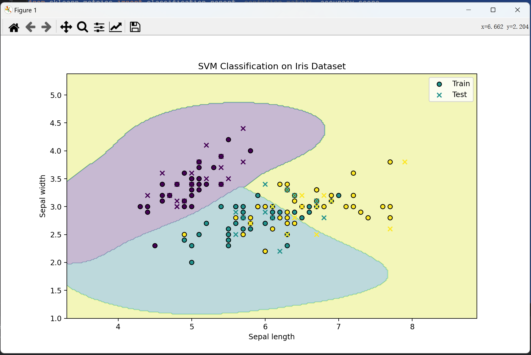
plt.contourf(xx, yy, Z, alpha=0.3)

# 绘制训练点
plt.scatter(X_train[:, 0], X_train[:, 1], c=y_train, edgecolors='k', label='Train')
plt.scatter(X_test[:, 0], X_test[:, 1], c=y_test, marker='x', label='Test')
plt.xlabel('Sepal length')
plt.ylabel('Sepal width')
plt.title('SVM Classification on Iris Dataset')
plt.legend()
plt.show()

• 运行效果图