CNN第四周 Art_Generation_with_Neural_Style_Transfer

深度学习在艺术上的应用：神经风格转换

Packages

import os
import sys
import scipy.io
import scipy.misc
import matplotlib.pyplot as plt
from matplotlib.pyplot import imshow
from PIL import Image
import numpy as np
import tensorflow as tf
from tensorflow.python.framework.ops import EagerTensor
import pprint
%matplotlib inline

Problem Statement

神经风格转换（Neural Style Transfer，NST）是深学习中最有趣的技术之一。如下图所示，它合并两个图像，即“内容”图像（C CContent）和“风格”图像（S SStyle），以创建“生成的”图像（G GGenerated）。生成的图像G将图像C的“内容”与图像S的“风格”相结合。

Transfer Learning

神经风格转换（NST）使用先前训练好了的卷积网络，并在此基础之上进行构建。使用在不同任务上训练的网络并将其应用于新任务的想法称为迁移学习。
根据原始的NST论文(https://arxiv.org/abs/1508.06576 )，我们将使用VGG网络，具体地说，我们将使用VGG-19，这是VGG网络的19层版本。这个模型已经在非常大的ImageNet数据库上进行了训练，因此学会了识别各种低级特征(浅层)和高级特征(深层)。

运行以下代码从VGG模型加载参数。这可能需要几秒钟。

tf.random.set_seed(272) # DO NOT CHANGE THIS VALUE
pp = pprint.PrettyPrinter(indent=4)
img_size = 400
vgg = tf.keras.applications.VGG19(include_top=False,
                                  input_shape=(img_size, img_size, 3),
                                  weights='pretrained-model/vgg19_weights_tf_dim_ordering_tf_kernels_notop.h5')

vgg.trainable = False
pp.pprint(vgg)

Neural Style Transfer (NST)

我们可以使用下面3个步骤来构建神经风格转换（Neural Style Transfer，NST）算法：

• 构建内容损失函数

• 构建风格损失函数

• 把它们放在一起

Computing the Content Cost

Make Generated Image G Match the Content of Image C

在执行NST时，您应该实现的一个目标是使生成的图像G中的内容与图像c的内容相匹配。要做到这一点，您需要了解浅层与深层的区别：

• 卷积神经网络较浅的层倾向于检测较低层次的特征，如边缘和简单纹理。
• 更深层的层倾向于检测更高级的特性，比如更复杂的纹理和对象类。

选择一个中间的激活层a[l]:

假设你选择了某一层来表示图像的内容，您需要“生成”的图像G与输入图像C内容要相似。

• 在实践中，如果你选择网络中间的一层——既不太浅也不太深，这样可以确保网络同时检测高层次和低层次的特性。会得到想要的结果。
• 在你完成了这个练习之后，可以自由地回来尝试使用不同的图层，看看结果是如何变化的!

前向传播图像C：

• 设图像C为预训练的VGG网络的输入，向前传播。
• 让a©成为选择图层隐藏层的激活，将是一个nH x nW x nC 的张量。

前向传播图像G：

• 对图像G重复这个过程:设置G为输入，并向前执行传播
• 让a(G)为被对应的隐藏层激活。

例子中，内容图片©是一张巴黎卢浮宫的图片

content_image = Image.open("images/louvre.jpg")
print("The content image (C) shows the Louvre museum's pyramid surrounded by old Paris buildings, against a sunny sky with a few clouds.")
content_image

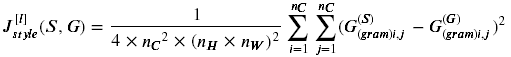
Content Cost Function Jcontent(C,G)

在执行NST时，你应该达到的一个目标是使生成的图像G中的内容与图像c中的内容相匹配。实现这一目标的方法是计算内容成本函数，其定义为:

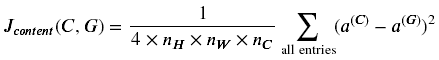
• 这里nH，nW,nC是指你选择隐藏层的高、宽、通道数，并出现在成本的归一化项中
• 为清楚期间，需要注意a©和a(G)是与隐藏层激活相对应的卷积值
• 为了计算成本Jcontent(C,G),可以方便的将3D卷积展开为2D
• 

Excercise 1 - compute_content_cost

计算内容代价函数
a_G：隐含层激活表示图像内容G
a_C：隐含层激活表示图像的内容

三步实现这个函数：

• 从a_G中获取维度信息
• 将a_G和a_C一样降维
• 计算内容代价

def compute_content_cost(content_output, generated_output):
    """
    Computes the content cost
    计算内容代价的函数
    Arguments:
    表示隐藏层中图像C的内容的激活值。
    a_C -- tensor of dimension (1, n_H, n_W, n_C), hidden layer activations representing content of the image C 
    表示隐藏层中图像G的内容的激活值。
    a_G -- tensor of dimension (1, n_H, n_W, n_C), hidden layer activations representing content of the image G
    
    Returns: 
    上面公式计算的值
    J_content -- scalar that you compute using equation 1 above.
    """
    a_C = content_output[-1]
    a_G = generated_output[-1]
    
    ### START CODE HERE
    
    # Retrieve dimensions from a_G (≈1 line)
    m, n_H, n_W, n_C = a_G.get_shape().as_list()
    
    # Reshape a_C and a_G (≈2 lines)
    # 先试用tf.reshape()将之前维度为(m,n_H,n_W,n_C)转换为(m, n_H * n_W, n_C)
    a_C_unrolled = tf.transpose(tf.reshape(a_C, shape=[m, n_H * n_W, n_C]))
    a_G_unrolled = tf.transpose(tf.reshape(a_G, shape=[m, n_H * n_W, n_C]))
    
    # compute the cost with tensorflow (≈1 line)
    J_content =  1/(4 * n_H * n_W * n_C)*tf.reduce_sum(tf.square(tf.subtract(a_C_unrolled, a_G_unrolled)))
    
    ### END CODE HERE
    
    return J_content

对于tf.shape()来说是获得张量维度大小的，而X.get_shape()是对于tensor的一个方法，返回的是一个元组，再使用.as_list()返回的是一个list
tf.transpose()是一个转置函数将tensor中的每个维度的位置进行转变

需要注意：

• 内容成本采用神经网络的隐层激活，并测量a ( C ) 与 a ( G ) 的区别。
• 当我们以后最小化内容成本时，这将有助于确保G 的内容与C 相似

Computing the Style Cost

下面是风格图像:

example = Image.open("images/monet_800600.jpg")
example

风格矩阵

风格矩阵又叫格拉姆矩阵(Gram matrix)。在线性代数中格拉姆矩阵G由一组向量(v1,…,vn)相互点乘(对应元素相乘)得到：

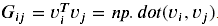
换句话说，Gij比较的是vi和vj的相似度，相似度越高，乘积越大，Gij就越大。

在神经风格转移(NST)中，我们可以利用展开矩阵和其转置矩阵相乘来计算格拉姆矩阵。

计算结果的格拉姆矩阵维度(nC, nC), 其中 nC 表示通道数(卷积核(filter)个数)。Gij的值表征的是filter i 的激活函数和filter j的激活函数的相似度。

格拉姆矩阵一个重要的部分是斜对角线上的元素Gii也表征了filter i 的活跃度。举个例子，假设 filter i 负责检测垂直纹理，则Gii表示了图片中垂直纹理的活跃度：Gii越大没标明图片中有越多的垂直纹理。

G中Gii表征了各个filter自己的普遍情况，Gij表征了不同filter共同作用的情况，这样G可以衡量一张图片的风格。

Exercise 2 - gram_matrix

def gram_matrix(A):
    """
    Argument:
    A -- matrix of shape (n_C, n_H*n_W)
    
    Returns:
    GA -- Gram matrix of A, of shape (n_C, n_C)
    """  
    ### START CODE HERE
    #(≈1 line)
    # 先对A做了转置，然后让A乘以A.T
    GA = tf.matmul(A, tf.transpose(A))
    ### END CODE HERE

    return GA

tf.matmul()函数与tf.multiply()的区别就是，第一个就是矩阵的乘法需要遵循矩阵乘法的规则，第二个是矩阵中对应元素相乘对应的是元素级的

Style Cost

你现在知道了如何计算出Gram矩阵，下一个目标就是最小化风格图像S的gram矩阵与生成图像G的gram矩阵的值
计算的公式如下所示:

Exercise 3 - compute_layer_style_cost

计算单个层的样本成本：以下三步:

• 得到隐藏层的激活a_G
• 将隐含层激活a_S和a_G展开成2D矩阵
• 计算图像S和G的Gram矩阵
• Compute the Style cost

def compute_layer_style_cost(a_S, a_G):
    """
    Arguments:
    隐藏层图像S的激活张量维度为(1,,n_H,n_W,n_C)
    a_S -- tensor of dimension (1, n_H, n_W, n_C), hidden layer activations representing style of the image S 
    a_G -- tensor of dimension (1, n_H, n_W, n_C), hidden layer activations representing style of the image G
    
    Returns: 
    返回值是每一层的风格代价
    J_style_layer -- tensor representing a scalar value, style cost defined above by equation (2)
    """
    ### START CODE HERE
    
    # Retrieve dimensions from a_G (≈1 line)
    m, n_H, n_W, n_C = a_G.get_shape().as_list()
    
    # Reshape the images from (n_H * n_W, n_C) to have them of shape (n_C, n_H * n_W) (≈2 lines)
    #得到经过转换平铺后的a_S和a_G
    a_S = tf.transpose(tf.reshape(a_S,[n_H * n_W, n_C]))
    a_G = tf.transpose(tf.reshape(a_G,[n_H * n_W, n_C]))

    # Computing gram_matrices for both images S and G (≈2 lines)
    # 得到的是图像的gram矩阵值
    GS = gram_matrix(a_S)
    GG = gram_matrix(a_G)
    
    # Computing the loss (≈1 line) 通过上面的公式带入
    J_style_layer = 1/(4* (n_C*n_C)* (n_H*n_W)*(n_H*n_W))*tf.reduce_sum(tf.square(tf.subtract(GS,GG)))
    
    ### END CODE HERE
    
    return J_style_layer

Style Weights

• 获取一层的style，想要得到更好的结果就必须结合风格代价多个不同的层
• 每一层都有一个权重去反应每一层对风格的影响
• 在默认情况下，每一层相等的权重加起来最后是1

Exercise 4 - compute_style_cost

计算风格代价

def compute_style_cost(style_image_output, generated_image_output, STYLE_LAYERS=STYLE_LAYERS):
    """
    Computes the overall style cost from several chosen layers
    计算从几个选择的层的总体风格代价
    Arguments:
    style_image_output -- our tensorflow model  我们的TensorFlow模型
    generated_image_output --
    STYLE_LAYERS -- A python list containing: 风格层
                        - the names of the layers we would like to extract style from
                        - a coefficient for each of them
    
    Returns: 
    J_style -- tensor representing a scalar value, style cost defined above by equation (2)
    """
    
    # initialize the overall style cost  初始化风格代价 
    J_style = 0

    # Set a_S to be the hidden layer activation from the layer we have selected.
    # 设置a_S为我们选择的隐藏层激活
    # The last element of the array contains the content layer image, which must not to be used.
    # 数组中最后的元素包含了内容层图像但不是一定会使用的
    a_S = style_image_output[:-1]

    # Set a_G to be the output of the choosen hidden layers.
    # The last element of the array contains the content layer image, which must not to be used.
    a_G = generated_image_output[:-1]
    for i, weight in zip(range(len(a_S)), STYLE_LAYERS):  
        # Compute style_cost for the current layer
        # 计算当前层的风格代价
        J_style_layer = compute_layer_style_cost(a_S[i], a_G[i])

        # Add weight * J_style_layer of this layer to overall style cost
        J_style += weight[1] * J_style_layer

    return J_style

如果你想生成的图像柔和地遵循风格图像，试着为更深的图层选择较大的权重，为第一层选择较小的权重。相反，如果您希望生成的图像强烈地遵循风格图像，请尝试为更深的层选择较小的权重，为第一层选择较大的权重。

注意：

• 图像的风格可以用隐藏层的激活的Gram矩阵来表示。
• 通过组合来自多个不同层的这种表示，可以得到更好的结果。
• 在内容表示中，通常只使用一个隐藏层就足够了。
• 最小化风格代价会使得图像G遵循图像S的风格。

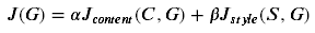
Defining the Total Cost to Optimize

最后将创造一个代价函数使得风格和内容代价最小，公式如下：

Exercise 5 - total_cost

@tf.function()
def total_cost(J_content, J_style, alpha = 10, beta = 40):
    """
    Computes the total cost function
    计算得到总体的代价函数
    Arguments:
    内容代价
    J_content -- content cost coded above
    风格代价
    J_style -- style cost coded above
    对于内容代价的超参数
    alpha -- hyperparameter weighting the importance of the content cost
    风格代价的超参数
    beta -- hyperparameter weighting the importance of the style cost
    
    Returns:
    J -- total cost as defined by the formula above.
    """
    ### START CODE HERE
    
    #(≈1 line)
    J = beta * J_style+alpha * J_content
    
    ### START CODE HERE

    return J

注意：

• 这总体的代价函数是一个线性的内容代价函数和风格代价函数
• α和β控制着内容和风格相关权重

Solving the Optimization Problem

最后，我们将各部分组合到一起实现神经风格迁移。
程序需要完成如下事情：

1. 载入内容图片
2. 载入风格图片
3. 随机初始化将要产生的图片
4. 载入VGG19模型
5. 计算内容代价
6. 计算风格代价
7. 计算整体代价
8. 定义优化器和学习率

Load the Content Image

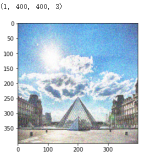
content_image = np.array(Image.open("images/louvre_small.jpg").resize((img_size, img_size)))
content_image = tf.constant(np.reshape(content_image, ((1,) + content_image.shape)))

print(content_image.shape)
imshow(content_image[0])
plt.show()

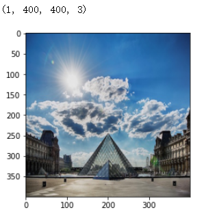
内容图像是(1,400,400,3)

Load the Style Image

style_image =  np.array(Image.open("images/monet.jpg").resize((img_size, img_size)))
style_image = tf.constant(np.reshape(style_image, ((1,) + style_image.shape)))

print(style_image.shape)
imshow(style_image[0])
plt.show()

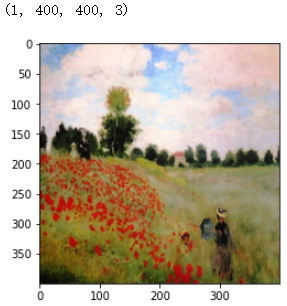
尺寸大小和内容图像一样

Randomly Initialize the Image to be Generated

现在需要将生成图像初始化为一个由内容图像创建的噪声图像

• 生成的图像与内容图像略有关联
• 通过初始化生成图像的像素，使大部分为噪声，但与内容图像略有关联，这将有助于生成图像内容更快速的匹配内容图像中的内容

generated_image = tf.Variable(tf.image.convert_image_dtype(content_image, tf.float32))
noise = tf.random.uniform(tf.shape(generated_image), 0, 0.5)
generated_image = tf.add(generated_image, noise)
generated_image = tf.clip_by_value(generated_image, clip_value_min=0.0, clip_value_max=1.0)

print(generated_image.shape)
imshow(generated_image.numpy()[0])
plt.show()

这是初始的生成图像。也就是结果图像。

Load Pre-trained VGG19 Model

定义一个函数，该函数加载VGG19模型，返回中间层的输出列表

def get_layer_outputs(vgg, layer_names):
    """ Creates a vgg model that returns a list of intermediate output values."""
    outputs = [vgg.get_layer(layer[0]).output for layer in layer_names]

    model = tf.keras.Model([vgg.input], outputs)
    return model

定义内容层并构建模型

content_layer = [('block5_conv4', 1)]

vgg_model_outputs = get_layer_outputs(vgg, STYLE_LAYERS + content_layer)

将内容和风格层的输出保存在单独的变量中

content_target = vgg_model_outputs(content_image)  # Content encoder
style_targets = vgg_model_outputs(style_image)     # Style enconder

Compute Total Cost

Compute Content Cost

构建模型后要计算内容代价，将a_C和a_G作为隐藏层激活。
将使用block5_conv4层来计算内容代价。下面代码执行以下操作：

• 设置a_C给隐藏层block5_conv4层作为激活
• 设置a_G作为激活与上面层数一致
• 使用a_C和a_G计算内容代价

# Assign the content image to be the input of the VGG model.  
# Set a_C to be the hidden layer activation from the layer we have selected
preprocessed_content =  tf.Variable(tf.image.convert_image_dtype(content_image, tf.float32))
a_C = vgg_model_outputs(preprocessed_content)

# Set a_G to be the hidden layer activation from same layer. Here, a_G references model['conv4_2'] 
# and isn't evaluated yet. Later in the code, we'll assign the image G as the model input.
a_G = vgg_model_outputs(generated_image)

# Compute the content cost 使用计算内容代价的函数
J_content = compute_content_cost(a_C, a_G)

print(J_content)

Compute Style Cost

# Assign the input of the model to be the "style" image 
preprocessed_style =  tf.Variable(tf.image.convert_image_dtype(style_image, tf.float32))
a_S = vgg_model_outputs(preprocessed_style)

# Compute the style cost
J_style = compute_style_cost(a_S, a_G)
print(J_style)

定义一些需要的函数，一个是截取张量中的0到1之间的像素。第二个函数是将张量转换为图像

def clip_0_1(image):
    """
    Truncate all the pixels in the tensor to be between 0 and 1
    截取在张量中介于0和1的像素
    Arguments:
    image -- Tensor
    J_style -- style cost coded above

    Returns:
    Tensor
    """
    return tf.clip_by_value(image, clip_value_min=0.0, clip_value_max=1.0)

def tensor_to_image(tensor):
    """
    Converts the given tensor into a PIL image
    将张量转换为一个PIL的图像
    Arguments:
    tensor -- Tensor
    
    Returns:
    Image: A PIL image
    """
    tensor = tensor * 255
    tensor = np.array(tensor, dtype=np.uint8)
    if np.ndim(tensor) > 3:
        assert tensor.shape[0] == 1
        tensor = tensor[0]
    return Image.fromarray(tensor)

Exercise 6 - train_step

实现迁移学习 train_step()函数：

• 使用Adam优化器去最小化总体代价J
• 学习率为：0.03
• 使用tf.GradientTape去更新图像

# 优化器 学习率为0.03
optimizer = tf.keras.optimizers.Adam(learning_rate=0.03)

@tf.function()
def train_step(generated_image):
    with tf.GradientTape() as tape:
        # In this function you must use the precomputed encoded images a_S and a_C
        # 使用之前预先编码的a_S和a_C
        # Compute a_G as the vgg_model_outputs for the current generated image
        # 计算a_G作为当前生成图像对于vgg模型的输出
        
        ### START CODE HERE
        
        #(1 line)
        a_G = vgg_model_outputs(generated_image)
        
        # Compute the style cost
        #(1 line)
        J_style = compute_style_cost(a_S, a_G)

        #(2 lines)
        # Compute the content cost
        J_content = compute_content_cost(a_C, a_G)
        # Compute the total cost
        J = total_cost(J_content, J_style, alpha = 10, beta = 40) 
        
        ### END CODE HERE
        
    grad = tape.gradient(J, generated_image)

    optimizer.apply_gradients([(grad, generated_image)])
    generated_image.assign(clip_0_1(generated_image))
    # For grading purposes
    return J

Train the Model

epochs = 2501
for i in range(epochs):
    train_step(generated_image)
    if i % 250 == 0:
        print(f"Epoch {i} ")
    if i % 250 == 0:
        image = tensor_to_image(generated_image)
        imshow(image)
        image.save(f"output/image_{i}.jpg")
        plt.show() 

会打印出来每隔250次训练得到的图像

#三个图像放在一块
# Show the 3 images in a row
fig = plt.figure(figsize=(16, 4))
ax = fig.add_subplot(1, 3, 1)
imshow(content_image[0])
ax.title.set_text('Content image')
ax = fig.add_subplot(1, 3, 2)
imshow(style_image[0])
ax.title.set_text('Style image')
ax = fig.add_subplot(1, 3, 3)
imshow(generated_image[0])
ax.title.set_text('Generated image')
plt.show()