1 Machine Learning Summary

本学习笔记参考自Andrew的机器学习课程(点此打开), 内容来自视频以及其讲义, 部分内容引用网友的学习笔记,会特别注明


课程前言


1.机器学习可以看到是很跨领域的,神经学,自然语言处理,等等,机器学习的实用性非常广
2.课程中的作业需要用到MATLAB软件编写实现一些学习算法,但是正版需要收费,OCTAVE是免费的,提供了一些跟MATLAB差不多的功能,但总的来说功能要少一些,不过对这门课程来说够用了 。

课程内容


一.机器学习定义(Machine Learning Definition)


Arthur Samuel: Field of study that gives computers the ability to learn without being explicitly programmed
这里Andrew举例Arthur Samuel的一个西洋棋程序例子,他的西洋棋程序可以自行学习如何下棋来战胜对方,但他并不是明显的写程序规则等来说明西洋棋应该如何去下棋,这个例子是上面定义的一个理解。
Tom Mitchell: A computer program is said to learn from experience E with respect to some task T and some performance measure P, if its performance on T, as measured by P, improves with experience E.

二.监督学习(supervised learning)


监督学习就是给算法提供了一套标准答案,让算法自行学习标准输入与标准输出答案之间的关联,以便来预测其他输入的输出。
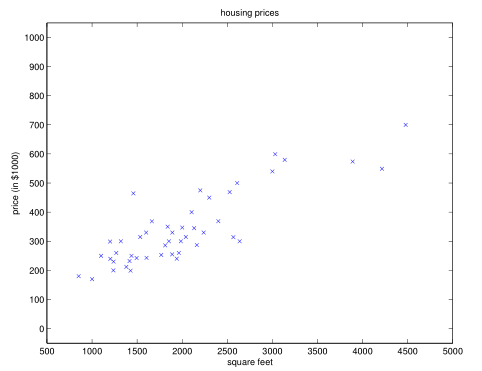
这里举例的是预测一个给定面积的房价,下面是图收集到的面积与房价的关系图,可以看做是现有的标注输入与答案。这其实也是一类回归问题,回归问题可以简单理解为如何去寻找多个自变量与因变量之间关系,即找出因变量与自变量之间的函数关系式

另一类监督学习问题是分类问题,分类问题处理的变量是离散的。这里举例为乳腺癌的性质(良性或恶性)与肿瘤大小的关系,其中肿瘤要么为良性要么为恶性,所以这里因变量是离散的,上面的回归问题的因变量是连续的,这是区别。这里也是通过给定肿瘤大小来预测是良性还是恶性,也就是分类。当然现实情况会复杂很多,不只是肿瘤的良性还是恶性会与多个因素相关,比如年龄,肿瘤大小等,这个时候的输入特征是二维的。如果输入特征向量是更多维的,那么就不能画图来表示出来了,有一种称为支持向量机(SVM)的算法是用来解决它的。

三.学习理论(learning theory)


这部分讲机器学习的理论以及算法介绍,比如你如何知道你的训练样本是否以及足够,,从Andrew的讲解来看,更重要的是机器学习的理念,原话是这样的:the skills to really take the learning algorithm ideas and really to get them to work on a problem

四.无监督学习(unsupervised learning)


无监督学习与监督学习的区别就是给你提供数据,但不给你提供正确答案。这里了很多例子,都是聚类,即给一组数据,然后将数据分成多个类别

五.强化学习(reinforcement learning)


强化学习的最基本的概念是回报函数的概念,需要找到一种方式去定义好的行为和坏的行为,用回报函数去奖励好的行为,惩罚坏的行为,用这种方式去学习

六.总结


上面的几个模块就是该课程内容后续将要仔细学习的内容


  • 1
    点赞
  • 0
    收藏
    觉得还不错? 一键收藏
  • 0
    评论
Okay, I understand your question. Here are the steps to answer it: Step 1: Select a dataset from the UCI Machine Learning Repository For this example, I will use the "Iris" dataset. This dataset contains information about the length and width of petals and sepals for three different species of Iris flowers. Step 2: Describe the dataset The "Iris" dataset contains 150 observations with four variables: sepal length, sepal width, petal length, and petal width. The dataset is commonly used in classification problems, as the goal is to predict the species of the flower based on its measurements. Step 3: Create a box plot with the lattice package To create a box plot with the lattice package, we first need to load the package and the dataset: ```R library(lattice) data(iris) ``` Next, we can create a box plot of the petal length by species: ```R bwplot(Petal.Length ~ Species, data = iris, main = "Boxplot of Petal Length by Species", xlab = "Species", ylab = "Petal Length") ``` Step 4: Analyse the graph The resulting box plot shows the distribution of petal length for each species of Iris flower. We can see that the "setosa" species has the shortest petals, while the "virginica" species has the longest petals. The "versicolor" species falls in between. Additionally, we can see that there are some outliers in the "versicolor" and "virginica" species, indicating that there may be some variability in petal length within those species. Overall, the box plot provides a visual summary of the distribution of petal length for each species of Iris flower, allowing us to quickly compare and contrast the different species.
评论
添加红包

请填写红包祝福语或标题

红包个数最小为10个

红包金额最低5元

当前余额3.43前往充值 >
需支付:10.00
成就一亿技术人!
领取后你会自动成为博主和红包主的粉丝 规则
hope_wisdom
发出的红包
实付
使用余额支付
点击重新获取
扫码支付
钱包余额 0

抵扣说明:

1.余额是钱包充值的虚拟货币,按照1:1的比例进行支付金额的抵扣。
2.余额无法直接购买下载,可以购买VIP、付费专栏及课程。

余额充值