python实现线性回归梯度下降法（吴恩达机器学习—笔记）

本人正在入门机器学习，到此来记一下笔记，还可以达到分享与被指点的效果，若哪里有问题或还可以优化，欢迎各位指正！

线性回归：

Hypothesis：假设函数

Cost Function：代价函数，即假设函数与数据集之间的误差

Goal：目标是找到参数、使代价函数的值最小，即误差最小

梯度下降：

梯度下降是一个用来求函数最小值的算法，我们将使用梯度下降算法来求出代价函数的最小值。

梯度下降的思想类似于：想象自己在一座山的某个位置，你要下山，但你不知道哪里是下山的路，那么有一个方法可以让你在这种情况下下山，那就是你在原点转一圈，找到比你目前所在的地势还要低的地方，找到即确定了方向，但我们还需要确定跨多大的步往这个方向走（即梯度下降法中所说的学习率），这些都确定后，迈出第一步到达地势较低的一点，如此重复以上步骤，直到你到达这座山的局部最低点。

转换一下：开始时我们随机选择一个参数的组合，计算代价函数，然后我们寻找下一个能让代价函数值下降最多的参数组合。我们持续这么做直到到到一个局部最小值（local minimum），因为我们并没有尝试完所有的参数组合，所以不能确定我们得到的局部最小值是否便是全局最小值（global minimum），选择不同的初始参数组合，可能会找到不同的局部最小值。

批量梯度下降（batch gradient descent）算法的公式为：

其中是学习率（learning rate），即如果步子太大了，可能会越过了最低点，如果步子太小了，则会下得慢。它决定了我们沿着能让代价函数下降程度最大的方向向下迈出的步子有多大，在批量梯度下降中，我们每一次都同时让所有的参数减去学习速率乘以代价函数的导数，以此来更新参数，参数必须要同时更新。

下面用python实现简单的线性回归梯度下降实验：

假设我们有数据集：，

假设函数：,         假设参数为：

由于在假设函数中，的系数为1，故在数据集最左中加上一列1，即：

代码如下：

import numpy as np
import matplotlib.pyplot as plt
def costFunctionJ(x,y,theta):
    '''代价函数'''
    m = np.size(x, axis = 0)
    predictions = x*theta
    sqrErrors = np.multiply((predictions - y),(predictions - y))
    j = 1/(2*m)*np.sum(sqrErrors)
    return j
 
def gradientDescent(x,y,theta,alpha,num_iters):
    '''
    alpha为学习率
    num_iters为迭代次数
    '''
    m = len(y)
    n = len(theta)
    temp = np.mat(np.zeros([n,num_iters]))  # 用来暂存每次迭代更新的theta值，是一个矩阵形式
    j_history = np.mat(np.zeros([num_iters,1]))     #  #记录每次迭代计算的代价值
    for i in range(num_iters):   # 遍历迭代次数
        h = x*theta
        #temp[0,i] = theta[0,0] - (alpha/m)*np.dot(x[:,1].T,(h-y)).sum()
        #temp[1,i] = theta[1,0] - (alpha/m)*np.dot(x[:,1].T,(h-y)).sum()
        temp[:,i] = theta - (alpha/m)*np.dot(x[:,1].T,(h-y)).sum()
        theta = temp[:,i]
        j_history[i] = costFunctionJ(x,y,theta)
    return theta,j_history,temp
 
x = np.mat([1,3,1,4,1,6,1,5,1,1,1,4,1,3,1,4,1,3.5,1,4.5,1,2,1,5]).reshape(12,2)
theta = np.mat([0,2]).reshape(2,1)
y = np.mat([1,2,3,2.5,1,2,2.2,3,1.5,3,1,3]).reshape(12,1)
 
# 求代价函数值
j = costFunctionJ(x,y,theta)
#print('代价值：',j)
 
plt.figure(figsize=(15,5))
plt.subplot(1,2,1)
plt.scatter(np.array(x[:,1])[:,0],np.array(y[:,0])[:,0],c='r',label='real data')  # 画梯度下降前的图像
plt.plot(np.array(x[:,1])[:,0],x*theta,label = 'test data')
plt.legend(loc = 'best')
plt.title('before')
 
theta, j_history, temp = gradientDescent(x,y,theta,0.01,100)
print('最终j_history值：\n',j_history[-1])
print('最终theta值：\n',theta)
print('每次迭代的代价值：\n',j_history)
print('theta值更新历史：\n',temp)
 
plt.subplot(1,2,2)
plt.scatter(np.array(x[:,1])[:,0],np.array(y[:,0])[:,0],c='r',label = 'real data')  # 画梯度下降后的图像
plt.plot(np.array(x[:,1])[:,0],x*theta,label = 'predict data')
plt.legend(loc = 'best')
plt.title('after')
plt.show()

运行结果：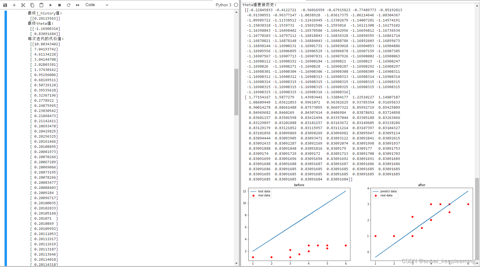

 

我们可以看到：

最终theta值：
 [[-1.16908316]
 [ 0.83091684]]

即参数、为-1,14和0.86使代价函数最小

欢迎指正！时刻保持谦逊好学。