Windows Caffe 学习笔记（四）搭建自己的网络，训练和测试MNIST手写字体库

本次笔记是学习官方文档“LeNet MNIST Tutorial”的记录，主要的收获是知道了如何去建立自己的训练和测试网络。其他步骤同之前的差不多，均进行的很顺利。

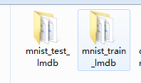
1.准备数据

也可以选择转换为LEVELDB，同之前的笔记中记录的一样，不再赘述。

2.搭建网络

这次搭建的网络，在原始的LeNet上做了一定改动。

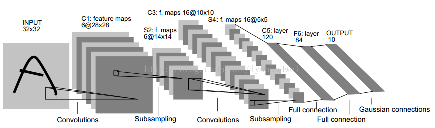
这是原始的LeNet模型图：

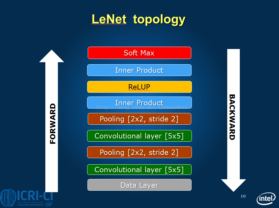
这次本次搭建的网络的模型图：

新建lenet_train__test_zlm.prototxt，下面为代码以及注释：

name:"LeNet"                 #命名

layer {
  name: "mnist"              # 输入层的名字为 mnist
  type: "Data"               # 输入的类型为 DATA
                             
                             #我们需要把输入像素灰度归一到【 0， 1），将 1 处以 256，得到 0.00390625。 
 transform_param {          
    scale: 0.00390625
  } 
                                  # 数据的参数 
  data_param {
    source: "examples/mnist/mnist_train_lmdb"    #从 mnist-train-lmdb 中读入数据
    backend: LMDB
    batch_size: 64                # 我们的批次大小为 64，即为了提高性能，一次处理 64 条数据
  }
  top: "data"                     # 这一层产生两个Blob，一个是data Blob，一个是label Blob
  top: "label"
   include {
    phase: TRAIN
  }
}

layer {
  name: "mnist"
  type: "Data"
  top: "data"
  top: "label"
  include {
    phase: TEST
  }
  transform_param {
    scale: 0.00390625
  }
  data_param {
    source: "examples/mnist/mnist_test_lmdb"
    batch_size: 100
    backend: LMDB
  }
}

layer {
  name: "conv1"                   # 卷积层名字为 conv1
  type: "Convolution"             # 类型为卷积
  param { lr_mult: 1 }            # 学习率调整的参数，我们设置权重学习率和运行中求解器给出的学习率一样，同时偏置学习率是其两倍
  param { lr_mult: 2 }            #lr_mults are the learning rate adjustments for the layer’s learnable parameters. In this case, 
                                  #we will set the weight learning rate to be the same as the learning rate given by the solver during runtime, 
                                  #and the bias learning rate to be twice as large as that - this usually leads to better convergence rates.
                                  # 卷积层的参数
  convolution_param {            
    num_output: 20                # 输出单元数 20
    kernel_size: 5                # 卷积核的大小为 5*5
    stride: 1                     # 步长为 1
                                  # 网络允许我们用随机值初始化权重和偏置值。   
   weight_filler {
      type: "xavier"              # 使用 xavier 算法自动确定基于输入和输出神经元数量的初始规模
    }
    bias_filler {
      type: "constant"            # 偏置值初始化为常数，默认为 0
    }
  }
  bottom: "data"                  # 这层前面使用 data，后面生成 conv1 的 Blob 空间
  top: "conv1"
}

layer {
  name: "pool1"                   #pooling 层名字叫 pool1
  type: "Pooling"                 #类型是 pooling
                                  #pooling 层的参数
 pooling_param {
    kernel_size: 2                #pooling 的核是 2X2
    stride: 2                     #pooling 的步长是 2
    pool: MAX                     #pooling 的方式是 MAX
  }
  bottom: "conv1"                 #这层前面使用 conv1,后面生层 pool1 的 Blob 空间
  top: "pool1"
}

layer {
  name: "conv2"
  type: "Convolution"
  bottom: "pool1"
  top: "conv2"
  param {
    lr_mult: 1
  }
  param {
    lr_mult: 2
  }
  convolution_param {
    num_output: 50               # 输出频道数 50
    kernel_size: 5           
    stride: 1
    weight_filler {
      type: "xavier"
    }
    bias_filler {
      type: "constant"
    }
  }
}

layer {
  name: "pool2"
  type: "Pooling"
  bottom: "conv2"
  top: "pool2"
  pooling_param {
    pool: MAX
    kernel_size: 2
    stride: 2
  }
}

layer {
  name: "ip1"                 # 全连接层的名字
  type: "InnerProduct"        # 类型是全连接层
  param { lr_mult: 1 }
  param { lr_mult: 2 }
                              # 全连接层的参数 
 inner_product_param {     
    num_output: 500           #输出 500 个节点，据说在一定范围内这里节点越多，正确率越高
    weight_filler {
      type: "xavier"
    }
    bias_filler {
      type: "constant"
    }
  }
  bottom: "pool2"
  top: "ip1"
}

layer {
  name: "relu1"
  type: "ReLU"               #类型是 RELU
  bottom: "ip1"              #Since ReLU is an element-wise operation, we can do in-place operations to save some memory.
  top: "ip1"                 #This is achieved by simply giving the same name to the bottom and top blobs. 
                             #Of course, do NOT use duplicated blob names for other layer types!
                             #由于是元素级的操作，我们可以现场激活来节省内存
}

layer {
  name: "ip2"
  type: "InnerProduct"
  param { lr_mult: 1 }
  param { lr_mult: 2 }
  inner_product_param {
    num_output: 10
    weight_filler {
      type: "xavier"
    }
    bias_filler {
      type: "constant"
    }
  }
  bottom: "ip1"
  top: "ip2"
}

layer {
  name: "accuracy"
  type: "Accuracy"
  bottom: "ip2"
  bottom: "label"
  top: "accuracy"
  include {
    phase: TEST
  }
}

layer {
  name: "loss"
  type: "SoftmaxWithLoss"
  bottom: "ip2"
  bottom: "label"          #It does not produce any outputs - all it does is to compute the loss function value, 
  #top: "loss"             #report it when backpropagation starts, and initiates the gradient with respect to ip2. 
                           #This is where all magic starts.`
}

注意：

<span style="color:#ff0000;">layer {
  // ...layer definition...
  include: { phase: TRAIN }
}</span>

下面是官方笔记的注解，就不做翻译了：

This is a rule, which controls layer inclusion in the network, based on current network’s state. You can refer to $CAFFE_ROOT/src/caffe/proto/caffe.proto for more information about layer rules and model schema.

In the above example, this layer will be included only in TRAIN phase. If we change TRAIN with TEST, then this layer will be used only in test phase. By default, that is without layer rules, a layer is always included in the network. Thus, lenet_train_test.prototxt has two DATA layers defined (with different batch_size), one for the training phase and one for the testing phase. Also, there is an Accuracy layer which is included only in TEST phase for reporting the model accuracy every 100 iteration, as defined in lenet_solver.prototxt.

3.编写求解文档

新建lenet_solver.prototxt，代码如下：

# The train/test net protocol buffer definition
net: "examples/mnist/lenet_train__test_zlm.prototxt"
# test_iter specifies how many forward passes the test should carry out.
# In the case of MNIST, we have test batch size 100 and 100 test iterations,
# covering the full 10,000 testing images.
test_iter: 100
# Carry out testing every 500 training iterations.
test_interval: 500
# The base learning rate, momentum and the weight decay of the network.
base_lr: 0.01
momentum: 0.9
weight_decay: 0.0005
# The learning rate policy
lr_policy: "inv"
gamma: 0.0001
power: 0.75
# Display every 100 iterations
display: 100
# The maximum number of iterations
max_iter: 10000
# snapshot intermediate results
snapshot: 5000
snapshot_prefix: "examples/mnist/lenet"
# solver mode: CPU or GPU
solver_mode: CPU

4.训练和测试

编写bat脚本，代码如下：

cd ../../
"Build/x64/Debug/caffe.exe" train --solver=examples/mnist/lenet_solver.prototxt
pause

运行bat文件，训练结果如下：

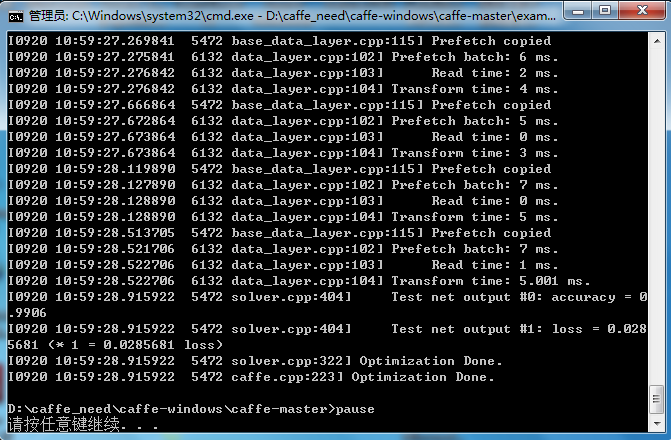
因为MNIST数据集很小，所以运行起来很快。最后的准确率0.9906，已经很高了，也说明模型是正确的。最后的损失值为0.0285681，也已经很小了。

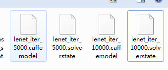
下面为迭代5000次和10000次得到的模型：

参考文档：

1.Caffe官方文档：LeNet MNIST Tutorial

2.学习笔记：Caffe上的LeNet模型理解