


%This program complished the process of 2D Eulerian advection with method
%of allocating memory temporarily.
clear all;clf;
% Set parameters
Nt = 1;
output_interval = 1;
Lx = 500000;
Ly = 500000;
Nx = 51;
Ny = 51;
Nx1 = Nx+1;
Ny1 = Ny+1;
dx = Lx / (Nx-1);
dy = Ly / (Ny-1);
% Basic E-nodes.
x = 0:dx:Lx;
y = 0:dy:Ly;
% Vx staggered nodes.(Nx_node * Ny_node+1)
xvx = 0:dx:Lx;
yvx = -dy/2 : dy : Ly+dy/2;
% Vy staggered nodes.(Nx_node+1 * Ny_node)
xvy = -dx/2 : dx : Lx+dx/2;
yvy = 0:dy:Ly;
% P staggered nodes.(Nx_node+1 * Ny_node+1)
xp = -dx/2 : dx : Lx+dx/2;
yp = -dy/2 : dy : Ly+dy/2;
vx_matrix = zeros(Ny1,Nx1);
vy_matrix = zeros(Ny1,Nx1);
pvx = zeros(Ny1,Nx1);
pvy = zeros(Ny1,Nx1);
vxp=zeros(Ny1,Nx1);
vyp=zeros(Ny1,Nx1);
p_matrix = zeros(Ny1,Nx1);
g_y = 10;
ETA = zeros(Ny,Nx);%density
RHO = zeros(Ny,Nx);%viscosity
% Amount of markers.
num_per_cell = 4;
Nx_marker = (Nx-1)*num_per_cell;
Ny_marker = (Ny-1)*num_per_cell;
marknum=Nx_marker*Ny_marker;
% Step-length among L-marker points
x_m_step = Lx/Nx_marker;
y_m_step = Ly/Ny_marker;
% Marker points.
xm=zeros(1,marknum); % Horizontal coordinates, m
ym=zeros(1,marknum);
rhom=zeros(1,marknum); % Density, kg/m^3
etam=zeros(1,marknum);
[X,Y] = meshgrid( x_m_step/2:x_m_step:Lx - x_m_step/2 , y_m_step/2:y_m_step:Ly - y_m_step/2 );
vis_marker = zeros(Ny_marker,Nx_marker);
den_marker = zeros(Ny_marker,Nx_marker);
den_plume = 3200;
radius = 100000;
den_mantle = 3300;
x_mid = Lx/2;
y_mid = Ly/2;
RHOVY=zeros(Ny1,Nx1); % Density in vy-nodes, kg/m^3
x_node = zeros(Ny_marker,Nx_marker);
y_node = zeros(Ny_marker,Nx_marker);
in_node = zeros(Ny+1,Nx+1);
in_vx = zeros(Ny+1,Nx+1);
in_vy = zeros(Ny+1,Nx+1);
in_p = zeros(Ny+1,Nx+1);
vx_markers = zeros(Ny_marker,Nx_marker);
vy_markers = zeros(Ny_marker,Nx_marker);
% Parameters and matrixs of exercise 9.3
srxy = zeros(Ny,Nx);
dsxy = zeros(Ny,Nx);
srxx = zeros(Ny,Nx);
dsxx = zeros(Ny,Nx);
pxyxy = zeros(Ny,Nx);
pxxxx = zeros(Ny,Nx);
Hs = zeros(Ny1,Nx1);
T = 1300;%K
aef = 3e-5;
Ha = zeros(Ny1,Nx1);
m = 1;
for jm=1:1:Nx_marker
for im=1:1:Ny_marker
% Define marker coordinates
xm(m)=x_m_step/2+(jm-1)*x_m_step+(rand-0.5)*x_m_step;
ym(m)=y_m_step/2+(im-1)*y_m_step+(rand-0.5)*y_m_step;
% Marker properties
rmark=((xm(m)-x_mid)^2+(ym(m)-y_mid)^2)^0.5;
if(rmark<=radius)
rhom(m)=3200; % Mantle density
etam(m)=1e+20; % Mantle viscosity
elseif(ym(m)<=0.2*Ly)
rhom(m)=1; % Sticky density
etam(m)=1e+17; % Sticky viscosity
else
rhom(m)=3300; % Plume density
etam(m)=1e+21; % Plume viscosity
end
% Update marker counter
m=m+1;
end
end
Kcont = 1e+21/dx;
dt=0e+12; % initial timestep
% Unknown_number is (Ny+1)*(Nx+1)*3
unknown_number = (Nx+1)*(Ny+1)*3;
coe = sparse(unknown_number,unknown_number);
R = zeros(unknown_number, 1);
% Boundary condition : free slip = -1 ; no slip = 1
bc_left = -1;
bc_right = -1;
bc_top = -1;
bc_bottom = -1;
dxymax = 0.5;
% Process of 2D transport
figure(1);
for t = 1:Nt
w_m_x_node = zeros(Ny,Nx);
den_w_m = zeros(Ny,Nx);
vis_w_m = zeros(Ny,Nx);
RHOYSUM=zeros(Ny1,Nx1);
WTYSUM=zeros(Ny1,Nx1);
% "drunken sailor" instability appear if dt = 0 at the next line.
% dt = 0;
% Interpolate density and viscosity from markers to BASIC NODES.
% Bisection algorithm
% Searching the coordinate of upper-left node of every L-marker.
for m=1:1:marknum
% Define i,j indexes for the upper left node
j=fix((xm(m)-x(1))/dx)+1;
i=fix((ym(m)-y(1))/dy)+1;
if(j<1)
j=1;
elseif(j>Nx-1)
j=Nx-1;
end
if(i<1)
i=1;
elseif(i>Ny-1)
i=Ny-1;
end
% Compute distances
dis_x = xm(m)-x(j);
dis_y = ym(m)-y(i);
wtmij = (1-dis_x/dx)*(1-dis_y/dy);
wtmi1j = (dis_x/dx)*(1-dis_y/dy);
wtmij1 = (1-dis_x/dx)*(dis_y/dy);
wtmi1j1 = (dis_x/dx)*(dis_y/dy);
% | |
% * * * * * Discard the m-point on the right.
w_m_x_node(i,j) = w_m_x_node(i,j) + wtmij;
den_w_m(i,j) = den_w_m(i,j) + rhom(m).*wtmij;
vis_w_m(i,j) = vis_w_m(i,j) + etam(m).*wtmij;
w_m_x_node(i+1,j) = w_m_x_node(i+1,j) + wtmi1j;
den_w_m(i+1,j) = den_w_m(i+1,j) + rhom(m).*wtmi1j;
vis_w_m(i+1,j) = vis_w_m(i+1,j) + etam(m).*wtmi1j;
w_m_x_node(i,j+1) = w_m_x_node(i,j+1) + wtmij1;
den_w_m(i,j+1) = den_w_m(i,j+1) + rhom(m).*wtmij1;
vis_w_m(i,j+1) = vis_w_m(i,j+1) + etam(m).*wtmij1;
w_m_x_node(i+1,j+1) = w_m_x_node(i+1,j+1) + wtmi1j1;
den_w_m(i+1,j+1) = den_w_m(i+1,j+1) + rhom(m).*wtmi1j1;
vis_w_m(i+1,j+1) = vis_w_m(i+1,j+1) + etam(m).*wtmi1j1;
% Density interpolation to vy-nodes
% Define i,j indexes for the upper left node
% Vy staggered nodes.(Nx_node+1 * Ny_node)
j=fix((xm(m)-xvy(1))/dx)+1;
i=fix((ym(m)-yvy(1))/dy)+1;
if(j<1)
j=1;
elseif(j>Nx)
j=Nx;
end
if(i<1)
i=1;
elseif(i>Ny-1)
i=Ny-1;
end
% Compute distances
dxmj=xm(m)-xvy(j);
dymi=ym(m)-yvy(i);
% Compute weights
wtmij=(1-dxmj/dx)*(1-dymi/dy);
wtmi1j=(1-dxmj/dx)*(dymi/dy);
wtmij1=(dxmj/dx)*(1-dymi/dy);
wtmi1j1=(dxmj/dx)*(dymi/dy);
% Update properties
% i,j Node
RHOYSUM(i,j)=RHOYSUM(i,j)+rhom(m)*wtmij;
WTYSUM(i,j)=WTYSUM(i,j)+wtmij;
% i+1,j Node
RHOYSUM(i+1,j)=RHOYSUM(i+1,j)+rhom(m)*wtmi1j;
WTYSUM(i+1,j)=WTYSUM(i+1,j)+wtmi1j;
% i,j+1 Node
RHOYSUM(i,j+1)=RHOYSUM(i,j+1)+rhom(m)*wtmij1;
WTYSUM(i,j+1)=WTYSUM(i,j+1)+wtmij1;
% i+1,j+1 Node
RHOYSUM(i+1,j+1)=RHOYSUM(i+1,j+1)+rhom(m)*wtmi1j1;
WTYSUM(i+1,j+1)=WTYSUM(i+1,j+1)+wtmi1j1;
end
% Computing the value of density and viscosity of E-nodes.
for j = 1:Nx
for i = 1:Ny
if(w_m_x_node(i,j)>0)
% Not need RHO on the basic nodes.Just Y nodes.
RHO(i,j) = den_w_m(i,j)/w_m_x_node(i,j);
ETA(i,j) = vis_w_m(i,j)/w_m_x_node(i,j);
end
end
end
for j=1:1:Nx1
for i=1:1:Ny1
if(WTYSUM(i,j)>0)
RHOVY(i,j)=RHOYSUM(i,j)/WTYSUM(i,j);
end
end
end
ETAP = zeros(Ny+1,Nx+1);
% Computing the harmonic density.
for j = 2:Nx
for i = 2:Ny
% Range of var_vis_n is 2:Ny 2:Nx.
ETAP(i,j) = 1/( (1/ETA(i,j) + 1/ETA(i-1,j) + 1/ETA(i,j-1) + 1/ETA(i-1,j-1) )/4 );
end
end
for j=1:1:Nx1
for i=1:1:Ny1
% Define global indexes in algebraic space
kvx=((j-1)*Ny1+i-1)*3+1; % Vx
kvy=kvx+1; % Vy
kpm=kvx+2; % P
% Vx equation External points
if(i==1 || i==Ny1 || j==1 || j==Nx || j==Nx1)
% Boundary Condition
% 1*Vx=0
coe(kvx,kvx)=1; % Left part
R(kvx)=0; % Right part
% Top boundary
if(i==1 && j>1 && j<Nx)
coe(kvx,kvx+3)=bc_top; % Left part
end
% Bottom boundary
if(i==Ny1 && j>1 && j<Nx)
coe(kvx,kvx-3)=bc_bottom; % Left part
end
else
% Internal points: x-Stokes eq.
% ETA*(d2Vx/dx^2+d2Vx/dy^2)-dP/dx=0
% Vx2
% |
% Vy1 | Vy3
% |
% Vx1-P1-Vx3-P2-Vx5
% |
% Vy2 | Vy4
% |
% Vx4
%
% Viscosity points
ETA1=ETA(i-1,j);
ETA2=ETA(i,j);
ETAP1=ETAP(i,j);
ETAP2=ETAP(i,j+1);
% Left part
coe(kvx,kvx-Ny1*3)=2*ETAP1/dx^2; % Vx1
coe(kvx,kvx-3)=ETA1/dy^2; % Vx2
coe(kvx,kvx)=-2*(ETAP1+ETAP2)/dx^2-(ETA1+ETA2)/dy^2; % Vx3
coe(kvx,kvx+3)=ETA2/dy^2; % Vx4
coe(kvx,kvx+Ny1*3)=2*ETAP2/dx^2; % Vx5
coe(kvx,kvy)=-ETA2/dx/dy; % Vy2
coe(kvx,kvy+Ny1*3)=ETA2/dx/dy; % Vy4
coe(kvx,kvy-3)=ETA1/dx/dy; % Vy1
coe(kvx,kvy+Ny1*3-3)=-ETA1/dx/dy; % Vy3
coe(kvx,kpm)=Kcont/dx; % P1
coe(kvx,kpm+Ny1*3)=-Kcont/dx; % P2
% Right part
R(kvx)=0;
end
% Vy equation External points
if(j==1 || j==Nx1 || i==1 || i==Ny || i==Ny1)
% Boundary Condition
% 1*Vy=0
coe(kvy,kvy)=1; % Left part
R(kvy)=0; % Right part
% Left boundary
if(j==1 && i>1 && i<Ny)
coe(kvy,kvy+3*Ny1)=bc_left; % Left part
end
% Right boundary
if(j==Nx1 && i>1 && i<Ny)
coe(kvy,kvy-3*Ny1)=bc_right; % Left part
end
else
% Internal points: y-Stokes eq.
% ETA*(d2Vy/dx^2+d2Vy/dy^2)-dP/dy=-RHO*gy
% Vy2
% |
% Vx1 P1 Vx3
% |
% Vy1----Vy3----Vy5
% |
% Vx2 P2 Vx4
% |
% Vy4
%
% Viscosity points
% Viscosity points
ETA1=ETA(i,j-1);
ETA2=ETA(i,j);
ETAP1=ETAP(i,j);
ETAP2=ETAP(i+1,j);
dRHOdx=(RHOVY(i,j+1)-RHOVY(i,j-1))/2/dx;
dRHOdy=(RHOVY(i+1,j)-RHOVY(i-1,j))/2/dy;
% Left part
coe(kvy,kvy-Ny1*3)=ETA1/dx^2; % Vy1
coe(kvy,kvy-3)=2*ETAP1/dy^2; % Vy2
coe(kvy,kvy)=-2*(ETAP1+ETAP2)/dy^2-...
(ETA1+ETA2)/dx^2 - dRHOdy*g_y*dt; % Vy3
coe(kvy,kvy+3)=2*ETAP2/dy^2; % Vy4
coe(kvy,kvy+Ny1*3)=ETA2/dx^2; % Vy5
coe(kvy,kvx)=-ETA2/dx/dy -dRHOdx*g_y*dt/4; %Vx3
coe(kvy,kvx+3)=ETA2/dx/dy -dRHOdx*g_y*dt/4; %Vx4
coe(kvy,kvx-Ny1*3)=ETA1/dx/dy -dRHOdx*g_y*dt/4; %Vx1
coe(kvy,kvx+3-Ny1*3)=-ETA1/dx/dy -dRHOdx*g_y*dt/4; %Vx2
coe(kvy,kpm)=Kcont/dy; % P1
coe(kvy,kpm+3)=-Kcont/dy; % P2
% Right part
R(kvy)=-RHOVY(i,j)*g_y;
end
% P equation External points
if(i==1 || j==1 || i==Ny1 || j==Nx1 ||...
(i==2 && j==2))
% Boundary Condition
% 1*P=0
coe(kpm,kpm)=1; % Left part
R(kpm)=0; % Right part
% Real BC
if(i==2 && j==2)
coe(kpm,kpm)=1*Kcont; %Left part
R(kpm)=1e+9; % Right part
end
else
% Internal points: continuity eq.
% dVx/dx+dVy/dy=0
% Vy1
% |
% Vx1--P--Vx2
% |
% Vy2
%
% Left part
coe(kpm,kvx-Ny1*3)=-1/dx; % Vx1
coe(kpm,kvx)=1/dx; % Vx2
coe(kpm,kvy-3)=-1/dy; % Vy1
coe(kpm,kvy)=1/dy; % Vy2
% Right part
R(kpm)=0;
end
end
end
% Computing the solution U:include vx,vy and p
U = coe \ R;
for j=1:1:Nx1
for i=1:1:Ny1
% Define global indexes in algebraic space
kvx=((j-1)*Ny1+i-1)*3+1; % Vx
kvy=kvx+1; % Vy
kpm=kvx+2; % P
% Reload solution
vx_matrix(i,j)=U(kvx);
vy_matrix(i,j)=U(kvy);
p_matrix(i,j)=U(kpm)*Kcont;
end
end
% Computing strain rate and deviatoric stress components.
for j = 1:Nx
for i = 1:Ny
srxy(i,j) = (1/2)*( (vx_matrix(i+1,j)-vx_matrix(i,j))/dy+(vy_matrix(i,j+1)-vy_matrix(i,j))/dx ) ;
dsxy(i,j) = 2*ETA(i,j)*srxy(i,j);
if(j~=1)
srxx(i,j) = ( vx_matrix(i,j)-vx_matrix(i,j-1) )/dx;
end
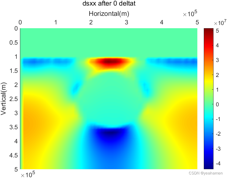
dsxx(i,j) = 2*ETAP(i,j)*srxx(i,j);
if(i~=1 && j~=1)
kxyxyij = srxy(i,j)*dsxy(i,j);
kxyxyi1j = srxy(i-1,j)*dsxy(i-1,j);
kxyxyij1 = srxy(i,j-1)*dsxy(i,j-1);
kxyxyi1j1 = srxy(i-1,j-1)*dsxy(i-1,j-1);
pxyxy(i,j) = (1/4)*(kxyxyij+kxyxyi1j+kxyxyij1+kxyxyi1j1);
kxxxxij = srxx(i,j)*dsxx(i,j);
kxxxxi1j = srxx(i-1,j)*dsxx(i-1,j);
kxxxxij1 = srxx(i,j-1)*dsxx(i,j-1);
kxxxxi1j1 = srxx(i-1,j-1)*dsxx(i-1,j-1);
pxxxx(i,j) = (1/4)*(kxxxxij+kxxxxi1j+kxxxxij1+kxxxxi1j1);
end
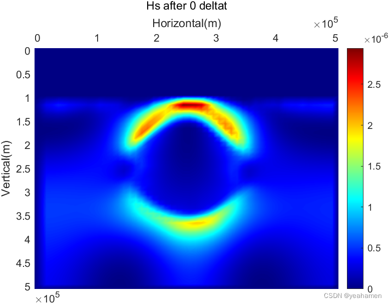
% Shear heating
Hs(i,j) = 2*( pxyxy(i,j) + pxxxx(i,j) ) ;
end
end
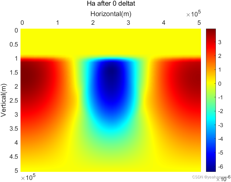
% Adiabatic heating
for j = 1:Nx1
for i = 2:Ny1
kvy = ( vy_matrix(i,j)+vy_matrix(i-1,j) )/2;
kRHO = ( RHOVY(i,j)+RHOVY(i-1,j) )/2;
Ha(i,j) = T*aef*g_y*kvy*kRHO;
end
end
% Computing average velocity components at cell centres.
for j = 1:Nx1
for i = 1:Ny1
% Computing internal Vx and Vy at the P nodes.
if (j~=1 && i ~=1 && j~=Nx1 && i~=Ny1)
% Vx at internal nodes.
pvx(i,j) = ( vx_matrix(i,j) + vx_matrix(i,j-1) )./2;
% Vy at internal nodes.
pvy(i,j) = ( vy_matrix(i,j) + vy_matrix(i-1,j) )./2;
end
end
end
% Why it is free-slip ??
% Applying free-slip boundary condition for velocity in the P nodes .
for j = 1:Nx1
for i = 1:Ny1
% j=1 j=2 j=3 ... j=Nx_node+1
% i=1
% i=2
% i=3
% ...
% i=Ny_node+1
if ( i==1 || i==Ny )
% Top and Bottom
% Vx
if(j>1 && j<Nx1)
pvx(i,j) = pvx(i+1,j);
end
% Vy
pvy(i,j) = pvy(i+1,j);
end
if (j==1 || j==Nx)
% Right and Left
% Vy
if(i>1 && i< Ny1)
pvy(i,j) = pvy(i,j+1);
end
% Vx
pvx(i,j) = pvx(i,j+1);
end
end
end
% Define time steps.
dt = 1e+36;
maxvx=max(max(abs(vx_matrix)));
maxvy=max(max(abs(vy_matrix)));
if(dt*maxvx>dxymax*dx)
dt=dxymax*dx/maxvx;
end
if(dt*maxvy>dxymax*dy)
dt=dxymax*dy/maxvy;
end
% The classical fourth-order Runge-Kutta scheme.
% Define Vxa(Vya)1,Vxb(Vyb)2,Vxc(Vyc)3,Vxd(Vyd)4.
vxm=zeros(4,1);
vym=zeros(4,1);
% Interpolate vx and vy components from E-nodes to L-markers.
for m=1:1:marknum
% Reserve original coordinate.
xa = xm(m);
ya = ym(m);
for rk = 1:1:4
% Interpolate vx from P-staggered nodes to L-markers.
% P staggered nodes.(Nx_node+1 * Ny_node+1)
j=fix((xm(m)-xp(1))/dx)+1;
i=fix((ym(m)-yp(1))/dy)+1;
if(j<1)
j=1;
elseif(j>Nx-1)
j=Nx-1;
end
% Vx staggered nodes.(Nx_node * Ny_node+1)
if(i<1)
i=1;
elseif(i>Ny)
i=Ny;
end
% Compute distances
dis_x=xm(m)-xp(j);
dis_y=ym(m)-yp(i);
% Compute weights
wtmij=(1-dis_x/dx)*(1-dis_y/dy);
wtmi1j=(dis_x/dx)*(1-dis_y/dy);
wtmij1=(1-dis_x/dx)*(dis_y/dy);
wtmi1j1=(dis_x/dx)*(dis_y/dy);
% Compute vx velocity
vxm(rk) = pvx(i,j)*wtmij+pvx(i+1,j)*wtmi1j...
+pvx(i,j+1)*wtmij1+pvx(i+1,j+1)*wtmi1j1;
vym(rk) = pvy(i,j)*wtmij+pvy(i+1,j)*wtmi1j...
+pvy(i,j+1)*wtmij1+pvy(i+1,j+1)*wtmi1j1;
% Interpolate vx from Vx-staggered nodes to L-markers.
% Define i,j indexes for the upper left node
j=fix((xm(m)-xvx(1))/dx)+1;
i=fix((ym(m)-yvx(1))/dy)+1;
if(j<1)
j=1;
elseif(j>Nx-1)
j=Nx-1;
end
% Vx staggered nodes.(Nx_node * Ny_node+1)
if(i<1)
i=1;
elseif(i>Ny)
i=Ny;
end
% Compute distances
dis_x=xm(m)-xvx(j);
dis_y=ym(m)-yvx(i);
% Compute weights
wtmij=(1-dis_x/dx)*(1-dis_y/dy);
wtmi1j=(dis_x/dx)*(1-dis_y/dy);
wtmij1=(1-dis_x/dx)*(dis_y/dy);
wtmi1j1=(dis_x/dx)*(dis_y/dy);
% Compute vx velocity
vxcij = (1/3)*(2*vx_matrix(i,j));
vxci1j = (1/3)*(2*vx_matrix(i+1,j));
vxcij1 = (1/3)*(2*vx_matrix(i,j+1));
vxci1j1 = (1/3)*(2*vx_matrix(i+1,j+1));
vxm(rk) = (1/3)*vxm(rk) + (vxcij*wtmij+vxci1j*wtmi1j...
+vxcij1*wtmij1+vxci1j1*wtmi1j1);
% Interpolate vy
% Define i,j indexes for the upper left node
j=fix((xm(m)-xvy(1))/dx)+1;
i=fix((ym(m)-yvy(1))/dy)+1;
if(j<1)
j=1;
elseif(j>Nx)
j=Nx;
end
if(i<1)
i=1;
elseif(i>Ny-1)
i=Ny-1;
end
% Compute distances
dis_x=xm(m)-xvy(j);
dis_y=ym(m)-yvy(i);
% Compute weights
wtmij=(1-dis_x/dx)*(1-dis_y/dy);
wtmi1j=(1-dis_x/dx)*(dis_y/dy);
wtmij1=(dis_x/dx)*(1-dis_y/dy);
wtmi1j1=(dis_x/dx)*(dis_y/dy);
% Compute vx velocity
vycij = (1/3)*(2*vy_matrix(i,j));
vyci1j = (1/3)*(2*vy_matrix(i+1,j));
vycij1 = (1/3)*(2*vy_matrix(i,j+1));
vyci1j1 = (1/3)*(2*vy_matrix(i+1,j+1));
vym(rk) = (1/3)*vym(rk) + (vycij*wtmij+vyci1j*wtmi1j...
+vycij1*wtmij1+vyci1j1*wtmi1j1);
if(rk == 1 || rk == 2)
xm(m) = vx_matrix(rk)*dt/2 + xa;
ym(m) = vy_matrix(rk)*dt/2 + ya;
elseif(rk == 3)
xm(m) = vx_matrix(rk)*dt + xa;
ym(m) = vy_matrix(rk)*dt + ya;
end
end
% Return original coordinate.
xm(m) = xa;
ym(m) = ya;
% Move markers
vxefft = (1/6)*(vxm(1)+2*vxm(2)+2*vxm(3)+vxm(4));
vyefft = (1/6)*(vym(1)+2*vym(2)+2*vym(3)+vym(4));
xm(m)=xm(m)+dt*vxefft;
ym(m)=ym(m)+dt*vyefft;
end
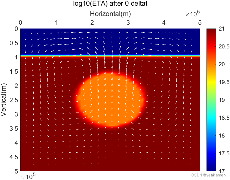
figure(1);
colormap('Jet');clf
pcolor(x,y,log10(ETA));
hold on;
%P nodes:(Nx+1 * Ny+1).
quiver(xp(1:2:Nx1),yp(1:2:Ny1),pvx(1:2:Ny1,1:2:Nx1),pvy(1:2:Ny1,1:2:Nx1),'w')
xlabel('Horizontal(m)')
ylabel('Vertical(m)')
caxis([17 21]);
set(gca,'xaxislocation','top');
set (gca,'YDir','reverse')
shading interp;
colorbar
title(['log10(ETA) after ',num2str(t-1),' deltat'])
pause(0.01);
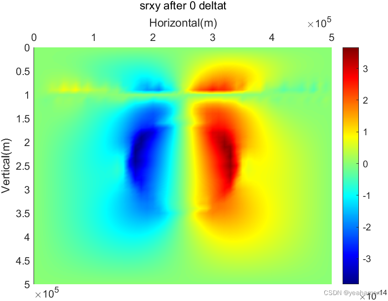
% Strain rate component:srxy
figure(2);
colormap('Jet');
pcolor(x(1:Ny),y(1:Nx),srxy);
xlabel('Horizontal(m)')
ylabel('Vertical(m)')
set(gca,'xaxislocation','top');
set (gca,'YDir','reverse')
shading interp;
colorbar
title(['srxy after ',num2str(t-1),' deltat'])
pause(0.01);
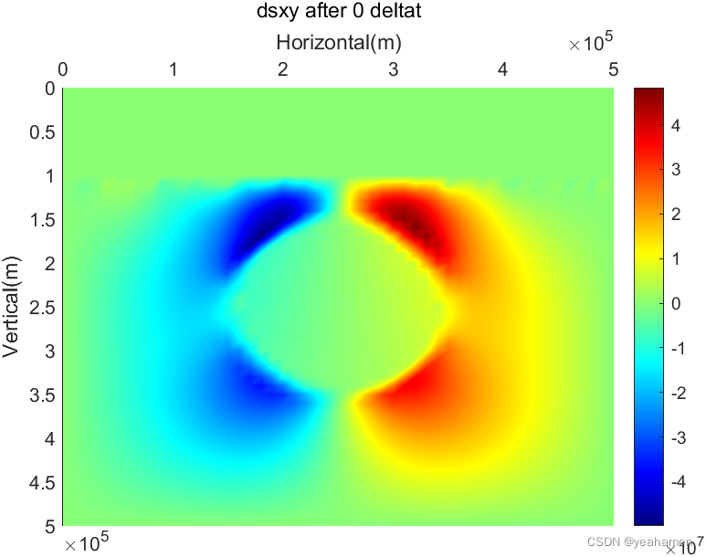
% Deviatoric stress component:srxy
figure(3);
colormap('Jet');
pcolor(x(1:Ny),y(1:Nx),dsxy);
xlabel('Horizontal(m)')
ylabel('Vertical(m)')
set(gca,'xaxislocation','top');
set (gca,'YDir','reverse')
shading interp;
colorbar
title(['dsxy after ',num2str(t-1),' deltat'])
pause(0.01);
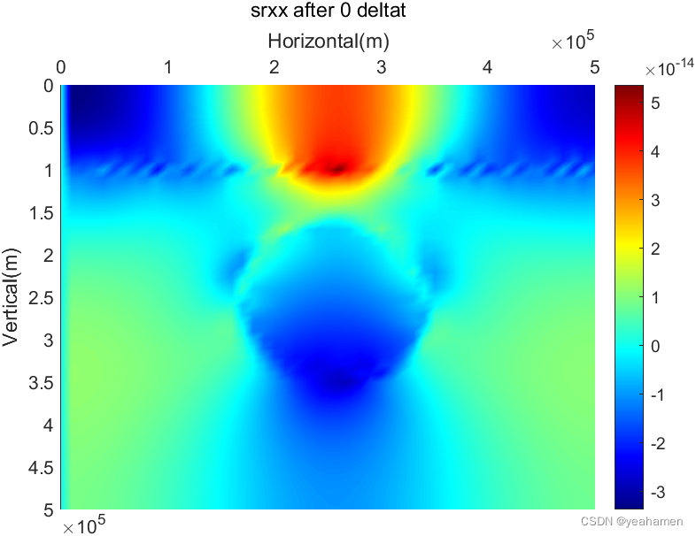
% Deviatoric stress component:srxy
figure(4);
colormap('Jet');
pcolor(x(1:Ny),y(1:Nx),srxx);
xlabel('Horizontal(m)')
ylabel('Vertical(m)')
set(gca,'xaxislocation','top');
set (gca,'YDir','reverse')
shading interp;
colorbar
title(['srxx after ',num2str(t-1),' deltat'])
pause(0.01);
% Deviatoric stress component:srxy
figure(5);
colormap('Jet');
pcolor(x(1:Ny),y(1:Nx),dsxx);
xlabel('Horizontal(m)')
ylabel('Vertical(m)')
set(gca,'xaxislocation','top');
set (gca,'YDir','reverse')
shading interp;
colorbar
title(['dsxx after ',num2str(t-1),' deltat'])
pause(0.01);
% Hs
figure(6);
colormap('Jet');
pcolor(xp,yp,Hs);
xlabel('Horizontal(m)')
ylabel('Vertical(m)')
set(gca,'xaxislocation','top');
set (gca,'YDir','reverse')
shading interp;
colorbar
title(['Hs after ',num2str(t-1),' deltat'])
pause(0.01);
% Hs
figure(7);
colormap('Jet');
pcolor(xp,yp,Ha);
xlabel('Horizontal(m)')
ylabel('Vertical(m)')
set(gca,'xaxislocation','top');
set (gca,'YDir','reverse')
shading interp;
colorbar
title(['Ha after ',num2str(t-1),' deltat'])
pause(0.01);
end


 4万+
4万+


 被折叠的 条评论
为什么被折叠?
被折叠的 条评论
为什么被折叠?
 到【灌水乐园】发言


