机器学习之SVM线性与非线性问题学习

---

第一部分：线性问题部分

import numpy as np

import matplotlib.pyplot as plt
%matplotlib inline

from sklearn.svm import SVC

import sklearn.datasets as datasets

1.1、生成随机散点

# 生成一序列的点，默认n_samples=100，中心centers=2
X,y = datasets.make_blobs(n_samples=50,centers=2)
X.shape #结果为(50, 2)

（1）查看X：

array([[10.19536929, -6.98207178],
       [ 8.17673749,  1.04956597],
       [ 7.11262117,  1.93567167],
       [ 7.69201225,  2.6067144 ],
       ... ...
       [ 9.7840538 , -5.97999583],
       [ 8.22020804,  2.17484189],
       [ 9.52555314, -7.75041062]])

（2）查看y：

array([0, 0, 0, 0, 1, 1, 0, 0, 0, 0, 1, 1, 1, 0, 1, 1, 1, 1, 1, 0, 1, 1,
       0, 0, 1, 0, 1, 0, 0, 1, 0, 0, 0, 1, 0, 0, 1, 0, 1, 1, 0, 0, 0, 1,
       1, 0, 1, 1, 1, 1])

---

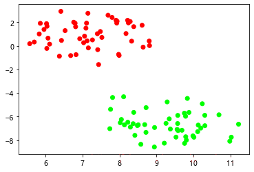
（3）画散点图：

#导入颜色
from matplotlib.colors import ListedColormap
color = ListedColormap([(1.0,0,0),(0,1.0,0)]) #红色和绿色

X,y = datasets.make_blobs(n_samples=100,centers=2) #生成100个散点，2个中心

plt.scatter(X[:,0],X[:,1],c = y,cmap = color) #散点图可视化

1.2、建模

• 现在需要画一条线把红色和绿色的点分隔开，先进行数据的学习，再确定这条线的截距和系数
• 线性回归方程： f(X) = w1*x1 + w2*x2 + b = x*w + b_
  • w = -w1/w2
  • b_ = -b/w2

svc = SVC(kernel='linear') #线性模型

svc.fit(X,y) #训练模型

（1）使用 svc.coef_ 获取该线的系数：

w1,w2 = svc.coef_[0]
print (svc.coef_)
print (w1)
print (w2)

[[ 0.14604164 -0.69448342]]
0.146041643741726
-0.6944834196263103

（2）使用 svc.intercept_ 获取截距：

b = svc.intercept_
b

array([-3.18503123])

（3）回归线 f(X) = w1*x1 + w2*x2 + b = x*w + b_ 推导：

（4）支持向量点直线：

• 支持向量点和分隔线平行，所以它们的斜率相等，当 f(x) = -1 和 f(x) = 1 时，可以求出通过支持向量点的两条直线；
• 公式：f(X) = x*w + b1 和 f(X) = x*w + b2
• 推导过程：

1 = w1*x + w2*y + b

-1 = w1*x + w2*y + b

b1 = -(b + 1)/w2

b2 = -(b - 1)/w2

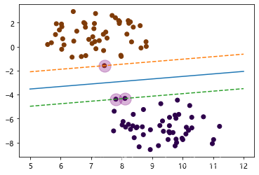
1.3、数据可视化

plt.scatter(X[:,0],X[:,1],c = y,cmap = plt.cm.PuOr) #原数据散点图

x = np.linspace(5,12,50) #这里的x值可以根据上面随机散点设置

#绘制回归线
plt.plot(x,x*w + b_)

#绘制支持向量点
plt.scatter(support_vectors_[:,0],support_vectors_[:,1],color = 'purple',s = 300,alpha = 0.3)

# 绘制两个支持向量点的直线
plt.plot(x,x*w + b1,ls = '--')
plt.plot(x,x*w + b2 ,ls = '--')

---

第二部分：非线性问题部分

import numpy as np

import matplotlib.pyplot as plt
%matplotlib inline

from sklearn.svm import SVC

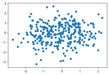
2.1、随机生成数据

X = np.random.randn(300,2) #生成300行2列的随机矩阵
X.shape #结果为(300,2)
plt.scatter(X[:,0],X[:,1]) #绘制散点图

---

2.2、属性组合分隔数据

• 可以通过数据的属性组合产生新的特征将数据区分出来，如通过它们的象限区分出来它们的属性；
• 第Ⅰ、Ⅲ象限相乘为正， 第Ⅱ、Ⅵ 相乘为负。

# 属性组合
# x3 = x1*x2
x3 = X[:,0] * X[:,1]
y = x3 >=0
#绘制散点图
plt.scatter(X[:,0],X[:,1],c = y)

---

2.3、建模

# rbf 径向基 高斯分布数据处理
svc = SVC(kernel='rbf')
svc.fit(X,y) #训练学习模型

2.3.1、测试范围

x1 = np.linspace(-3,3,100)
y1 = np.linspace(-3,3,100)
X1,Y1 = np.meshgrid(x1,y1) #网格交叉，X1和Y1都是(100, 100)的矩阵了

#散点图可视化
X_test = np.concatenate([X1.reshape(-1,1),Y1.reshape(-1,1)],axis=-1) #concatenate数据集联
plt.scatter(X_test[:,0],X_test[:,1])

结果分析： 这是结果是正确的。因为这上面有10000个点，分布太多密集。

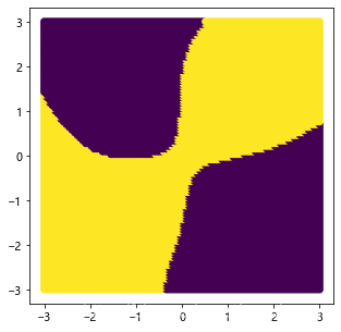
2.3.2、预测分隔

y_ = svc.predict(X_test) #预测测试

plt.figure(figsize=(5,5)) #设置图像比例

plt.scatter(X_test[:,0],X_test[:,1],c = y_) #作散点图

2.3.3、求它的距离

d_ = svc.decision_function(X_test)
d_

array([0.1093417 , 0.11477454, 0.12075184, ..., 0.16816356, 0.16268286,
       0.15759471])

绘制轮廓面：

plt.figure(figsize=(5,5))

plt.contourf(X1,Y1,d_.reshape(100,100)) #轮廓面contourf

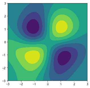
结果分析： 颜色越深，说明值越大，离分离超平面越远。

第三部分：SVM回归实战

3.1、准备数据

import numpy as np

import matplotlib.pyplot as plt
%matplotlib inline

from sklearn.svm import SVR

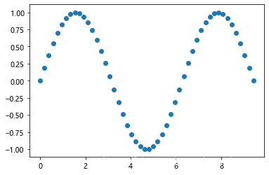
X = np.linspace(0,3*np.pi,50).reshape(-1,1) #转化为二维数据
y = np.sin(X)

plt.scatter(X,y) #画散点图

---

3.2、建立模型

svr_linear  = SVR(kernel='linear') #线性

svr_rbf = SVR(kernel='rbf') #高斯

svr_poly = SVR(kernel='poly') #多项式

svr_linear.fit(X,y)

svr_rbf.fit(X,y)

svr_poly.fit(X,y)

---

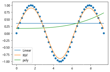
3.3、预测数据及可视化

# 生成测试集
X_test = np.linspace(0, 3*np.pi, 128).reshape(-1,1)

#在模型中预测目标
y1 = svr_linear.predict(X_test) #线性

y2 = svr_rbf.predict(X_test) #高斯

y3 = svr_poly.predict(X_test) #多项式

#可视化
plt.scatter(X,y) #原散点图

plt.plot(X_test,y1)

plt.plot(X_test,y2)

plt.plot(X_test,y3)

plt.legend(['Linear','Rbf','poly']) #显示标签