


记录机器学习中涉及的代码...
1. 线性回归分析
分析对象
生成 y=4+3*x函数的随机值,采用梯度下降算法进行代价函数计算。
计算程序
import numpy as np
import matplotlib.pyplot as plt

# 生成一些模拟数据
np.random.seed(0)
X = 2 * np.random.rand(100, 1)
y = 4 + 3 * X + np.random.randn(100, 1)

# 在 X 前添加一列,用于计算截距
X_b = np.c_[np.ones((100, 1)), X]

# 设置梯度下降的参数
eta = 0.001  # 学习率
n_iterations = 1000

# 随机初始化参数
theta = np.random.randn(2, 1)

# 初始化一个数组用于存储每次迭代的代价函数值
cost_history = np.zeros(n_iterations)

# 使用梯度下降算法求解参数
for iteration in range(n_iterations):
    # 计算梯度
    gradients = 2/100 * X_b.T.dot(X_b.dot(theta) - y)
    # 更新参数
    theta = theta - eta * gradients
    # 计算代价函数并存储
    cost = np.mean((X_b.dot(theta) - y) ** 2)
    cost_history[iteration] = cost

# 打印最终的参数
print("最终参数(theta):", theta)

# 绘制原始数据和拟合的直线
plt.scatter(X, y)
plt.plot(X, X_b.dot(theta), 'r-')
plt.xlabel('X')
plt.ylabel('y')
plt.title('Linear Regression with Gradient Descent')

# 绘制代价函数计算结果曲线
plt.figure()
plt.plot(range(1, n_iterations + 1), cost_history, color='blue')
plt.xlabel('Iterations')
plt.ylabel('Cost')
plt.title('Cost Function Over Iterations')

plt.show()
运行结果
theta参数为:
[[3.86291512] [3.15339547]]


说明
np.c_是 NumPy 中的一个类,它用于按列连接两个矩阵,类似于np.column_stack。在上述代码中,np.c_用于在生成的随机数据X中添加一列偏置项,这是 logistic 回归中常用的操作。-
np.hstack是 NumPy 中的函数,用于在水平方向上(按列)堆叠数组。具体而言,np.hstack将两个数组水平堆叠在一起,形成一个新的数组。在上述代码中,np.hstack((np.ones((num_samples, 1)), X))的目的是在数据集X的左侧添加一列全为 1 的列,即添加偏置项,以便在模型中使用。这是为了表示线性方程中的截距项。 - 在代码的开头使用
np.random.seed(0)是为了确保在生成随机数据时得到可重复的结果。通过设置随机种子(seed),可以使得每次运行程序时生成的随机数相同,这对于调试和验证代码的结果很有帮助。如果省略了np.random.seed(0),每次运行程序时都会得到不同的随机数据,这可能导致结果的不确定性。
2. Logistic分析
分析对象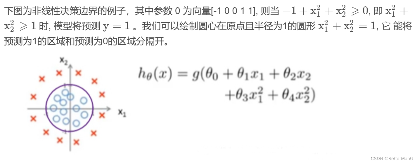
计算程序
import numpy as np
import matplotlib.pyplot as plt
from mpl_toolkits.mplot3d import Axes3D

# 步骤1:生成数据集
np.random.seed(0)
num_samples = 100
# 在范围[-1, 1]内生成随机数据
X = np.random.rand(num_samples, 2) * 2 - 1
# 如果 x1**2 + x2**2 小于1.0,则设置 y=1.0,否则设置 y=0.0
y = (X[:, 0]**2 + X[:, 1]**2 < 1.0).astype(float)

# 步骤2:定义逻辑函数及其梯度
def sigmoid(z):
    return 1.0 / (1.0 + np.exp(-z))

def sigmoid_gradient(z):
    return sigmoid(z) * (1 - sigmoid(z))

# 步骤3:实现梯度下降
def gradient_descent(X, y, learning_rate, num_iterations):
    num_samples, num_features = X.shape
    # 添加偏置列和输入特征的平方列
    X = np.hstack((np.ones((num_samples, 1)), X, np.square(X)))

    # 初始化参数
    theta = np.zeros(num_features + 2 + 1)  # 包括偏置项和平方项

    # 记录每次迭代的代价
    costs = []

    for _ in range(num_iterations):
        # 计算预测值
        predictions = sigmoid(np.dot(X, theta))

        # 计算代价函数
        cost = -np.mean(y * np.log(predictions) + (1 - y) * np.log(1 - predictions))
        costs.append(cost)

        # 计算梯度
        gradient = np.dot(X.T, (predictions - y)) / num_samples

        # 更新参数
        theta -= learning_rate * gradient

    return theta, costs

# 步骤4:绘制代价函数曲线和决策边界
def plot_results(X, y, theta, costs):
    fig = plt.figure(figsize=(12, 8))

    # 绘制代价函数曲线
    ax1 = fig.add_subplot(221)
    ax1.plot(costs)
    ax1.set_title('Cost Function')

    # 绘制数据点
    ax2 = fig.add_subplot(222, projection='3d')
    ax2.scatter(X[:, 0], X[:, 1], y, c=y, cmap='viridis')
    ax2.set_title('Data Points')

    # 绘制决策边界
    ax3 = fig.add_subplot(223, projection='3d')
    x1_vals, x2_vals = np.meshgrid(np.linspace(-1, 1, 100), np.linspace(-1, 1, 100))
    X_vals = np.c_[x1_vals.flatten(), x2_vals.flatten()]
    X_vals = np.hstack((np.ones((X_vals.shape[0], 1)), X_vals, np.square(X_vals)))
    decision_boundary = sigmoid(np.dot(X_vals, theta))
    decision_boundary = decision_boundary.reshape(x1_vals.shape)
    ax3.plot_surface(x1_vals, x2_vals, decision_boundary, cmap='viridis', alpha=0.5)
    ax3.scatter(X[:, 0], X[:, 1], y, c=y, cmap='viridis')
    ax3.set_title('Decision Boundary')
    plt.show()

# 运行梯度下降
learning_rate = 0.1
num_iterations = 20000
theta, costs = gradient_descent(X, y, learning_rate, num_iterations)

# 打印学到的参数
print(theta)

# 绘制结果
plot_results(X, y, theta, costs)

# 说明:
#
# 数据生成:在范围[-1, 1]内生成随机数据,并根据一个圆形区域分配标签。
# 逻辑函数:定义逻辑函数及其梯度,用于逻辑回归。
# 梯度下降:实现梯度下降,优化逻辑回归参数。
# 绘图结果:绘制代价函数曲线、数据点和决策边界的三维图。
运行结果
theta参数为:
[ 12.34895505 0.68837517 -0.0789526 -11.50124612 -13.1030072 ]

3. Logistic分析,采用正则化
分析对象
计算程序
import numpy as np
import matplotlib.pyplot as plt
from mpl_toolkits.mplot3d import Axes3D

# 步骤1:生成数据集
np.random.seed(0)
num_samples = 1000
X = np.random.rand(num_samples, 2) * 2 - 1  # 生成在[-1, 1]范围内的随机数据
y = (X[:, 0]**2 + X[:, 1]**2 < 1.0).astype(float)

# 步骤2:定义 logistic 函数及其梯度
def sigmoid(z):
    return 1.0 / (1.0 + np.exp(-z))

def sigmoid_gradient(z):
    return sigmoid(z) * (1 - sigmoid(z))

# 步骤3:实现带有 L2 正则化的梯度下降
def gradient_descent_with_regularization(X, y, learning_rate, num_iterations, alpha):
    num_samples, num_features = X.shape
    X = np.hstack((np.ones((num_samples, 1)), X, np.square(X)))  # 添加一列偏置项

    # 初始化参数
    theta = np.zeros(num_features + 2 + 1)

    # 记录每次迭代的代价
    costs = []

    for _ in range(num_iterations):
        # 计算预测值
        predictions = sigmoid(np.dot(X, theta))

        # 计算带有正则化的代价函数
        cost = -np.mean(y * np.log(predictions) + (1 - y) * np.log(1 - predictions)) + (alpha / (2 * num_samples)) * np.sum(theta[1:]**2)
        costs.append(cost)

        # 计算梯度
        gradient = (np.dot(X.T, (predictions - y)) + alpha * np.hstack((0, theta[1:]))) / num_samples

        # 更新参数
        theta -= learning_rate * gradient

    return theta, costs

# 步骤4:绘制代价函数曲线和决策边界
def plot_results(X, y, theta, costs):
    fig = plt.figure(figsize=(12, 8))

    # 绘制代价函数曲线
    ax1 = fig.add_subplot(221)
    ax1.plot(costs)
    ax1.set_title('Cost Function')

    # 绘制数据点
    ax2 = fig.add_subplot(222, projection='3d')
    ax2.scatter(X[:, 0], X[:, 1], y, c=y, cmap='viridis')
    ax2.set_title('Data Points')

    # 绘制决策边界
    ax3 = fig.add_subplot(223, projection='3d')
    x1_vals, x2_vals = np.meshgrid(np.linspace(-1, 1, 100), np.linspace(-1, 1, 100))
    X_vals = np.c_[x1_vals.flatten(), x2_vals.flatten()]
    X_vals = np.hstack((np.ones((X_vals.shape[0], 1)), X_vals, np.square(X_vals)))
    decision_boundary = sigmoid(np.dot(X_vals, theta))
    decision_boundary = decision_boundary.reshape(x1_vals.shape)
    ax3.plot_surface(x1_vals, x2_vals, decision_boundary, cmap='viridis', alpha=0.5)
    ax3.scatter(X[:, 0], X[:, 1], y, c=y, cmap='viridis')
    ax3.set_title('Decision Boundary')
    plt.show()

# 运行梯度下降(使用正则化)
learning_rate = 0.1
num_iterations = 20000
alpha = 10 # 正则化参数
theta, costs = gradient_descent_with_regularization(X, y, learning_rate, num_iterations, alpha)

# 打印学到的参数
print(theta)

# 绘制结果
plot_results(X, y, theta, costs)
运行结果
随着正则参数增加,theta参数逐渐变小。样本数量越多,代价函数最终值也会越低。
theta参数:
[ 3.47261718 -0.06700464 -0.06413931 -2.89488142 -2.78282584]


 939
939

 被折叠的 条评论
为什么被折叠?
被折叠的 条评论
为什么被折叠?
 到【灌水乐园】发言


