


{作为CNN学习入门的一部分,笔者在这里逐步给出UFLDL的各章节Exercise的个人代码实现,供大家参考指正}
理论部分可以在线参阅(页面最下方有中文选项)Self-Taught Learning章节的内容。
Notes:
1. 整个过程只是将之前几章节的Assignment总结了一下,加以运用。
关键在于对之前用过的函数的参数的理解,这里需要根据Input的不同,对函数输入参数进行调整。详情请参阅下文代码。
2. 需要理解无监督学习对特征的提取过程,然后在有监督学习时也用同样的方法提取特征,进而将特征输入softmax分类器。
stlExercise.m
%% CS294A/CS294W Self-taught Learning Exercise

%  Instructions
%  ------------
%
%  This file contains code that helps you get started on the
%  self-taught learning. You will need to complete code in feedForwardAutoencoder.m
%  You will also need to have implemented sparseAutoencoderCost.m and
%  softmaxCost.m from previous exercises.
%
%% ======================================================================
%  STEP 0: Here we provide the relevant parameters values that will
%  allow your sparse autoencoder to get good filters; you do not need to
%  change the parameters below.

inputSize  = 28 * 28;
numLabels  = 5;
hiddenSize = 200;
sparsityParam = 0.1; % desired average activation of the hidden units.
                     % (This was denoted by the Greek alphabet rho, which looks like a lower-case "p",
		             %  in the lecture notes).
lambda = 3e-3;       % weight decay parameter
beta = 3;            % weight of sparsity penalty term
maxIter = 400;

%% ======================================================================
%  STEP 1: Load data from the MNIST database
%
%  This loads our training and test data from the MNIST database files.
%  We have sorted the data for you in this so that you will not have to
%  change it.

% Load MNIST database files
mnistData   = loadMNISTImages('mnist/train-images.idx3-ubyte');
mnistLabels = loadMNISTLabels('mnist/train-labels.idx1-ubyte');

% Set Unlabeled Set (All Images)

% Simulate a Labeled and Unlabeled set
labeledSet   = find(mnistLabels >= 0 & mnistLabels <= 4);
unlabeledSet = find(mnistLabels >= 5);

numTrain = round(numel(labeledSet)/2);
trainSet = labeledSet(1:numTrain);
testSet  = labeledSet(numTrain+1:end);

unlabeledData = mnistData(:, unlabeledSet);

trainData   = mnistData(:, trainSet);
trainLabels = mnistLabels(trainSet)' + 1; % Shift Labels to the Range 1-5

testData   = mnistData(:, testSet);
testLabels = mnistLabels(testSet)' + 1;   % Shift Labels to the Range 1-5

% Output Some Statistics
fprintf('# examples in unlabeled set: %d\n', size(unlabeledData, 2));
fprintf('# examples in supervised training set: %d\n\n', size(trainData, 2));
fprintf('# examples in supervised testing set: %d\n\n', size(testData, 2));

%% ======================================================================
%  STEP 2: Train the sparse autoencoder
%  This trains the sparse autoencoder on the unlabeled training
%  images.

%  Randomly initialize the parameters
theta = initializeParameters(hiddenSize, inputSize);

%% ----------------- YOUR CODE HERE ----------------------
%  Find opttheta by running the sparse autoencoder on
%  unlabeledTrainingImages

%  opttheta = theta;

 patches = unlabeledData;

 %  Use minFunc to minimize the function
 addpath minFunc/
 options.Method = 'lbfgs'; % Here, we use L-BFGS to optimize our cost
                           % function. Generally, for minFunc to work, you
                           % need a function pointer with two outputs: the
                           % function value and the gradient. In our problem,
                           % sparseAutoencoderCost.m satisfies this.
 options.maxIter = 400;	  % Maximum number of iterations of L-BFGS to run
 options.display = 'on';

 [opttheta, cost] = minFunc( @(p) sparseAutoencoderCost(p, ...
                                    inputSize, hiddenSize, ...
                                    lambda, sparsityParam, ...
                                    beta, patches), ...
                               theta, options);

%% -----------------------------------------------------

% Visualize weights
W1 = reshape(opttheta(1:hiddenSize * inputSize), hiddenSize, inputSize);
display_network(W1');

%%======================================================================
%% STEP 3: Extract Features from the Supervised Dataset
%
%  You need to complete the code in feedForwardAutoencoder.m so that the
%  following command will extract features from the data.

trainFeatures = feedForwardAutoencoder(opttheta, hiddenSize, inputSize, ...
                                       trainData);

testFeatures = feedForwardAutoencoder(opttheta, hiddenSize, inputSize, ...
                                       testData);

%%======================================================================
%% STEP 4: Train the softmax classifier

softmaxModel = struct;
%% ----------------- YOUR CODE HERE ----------------------
%  Use softmaxTrain.m from the previous exercise to train a multi-class
%  classifier.

%  Use lambda = 1e-4 for the weight regularization for softmax

% You need to compute softmaxModel using softmaxTrain on trainFeatures and
% trainLabels
lambda = 1e-4;

% Randomly initialise theta
theta = 0.005 * randn(numLabels * hiddenSize, 1);

%  Implement softmaxCost in softmaxCost.m.
[cost, grad] = softmaxCost(theta, numLabels, hiddenSize, lambda, trainFeatures, trainLabels);

options.maxIter = 100;
softmaxModel = softmaxTrain(hiddenSize, numLabels, lambda, ...
                            trainFeatures, trainLabels, options);

%% -----------------------------------------------------


%%======================================================================
%% STEP 5: Testing

%% ----------------- YOUR CODE HERE ----------------------
% Compute Predictions on the test set (testFeatures) using softmaxPredict
% and softmaxModel


% You will have to implement softmaxPredict in softmaxPredict.m
[pred] = softmaxPredict(softmaxModel, testFeatures);

%% -----------------------------------------------------

% Classification Score
fprintf('Test Accuracy: %f%%\n', 100*mean(pred(:) == testLabels(:)));

% (note that we shift the labels by 1, so that digit 0 now corresponds to
%  label 1)
%
% Accuracy is the proportion of correctly classified images
% The results for our implementation was:
%
% Accuracy: 98.3%
% My Accuracy: 98.221990%
%
function [activation] = feedForwardAutoencoder(theta, hiddenSize, visibleSize, data)

% theta: trained weights from the autoencoder
% visibleSize: the number of input units (probably 64)
% hiddenSize: the number of hidden units (probably 25)
% data: Our matrix containing the training data as columns.  So, data(:,i) is the i-th training example.

% We first convert theta to the (W1, W2, b1, b2) matrix/vector format, so that this
% follows the notation convention of the lecture notes.

W1 = reshape(theta(1:hiddenSize*visibleSize), hiddenSize, visibleSize);
b1 = theta(2*hiddenSize*visibleSize+1:2*hiddenSize*visibleSize+hiddenSize);

%% ---------- YOUR CODE HERE --------------------------------------
%  Instructions: Compute the activation of the hidden layer for the Sparse Autoencoder.
activation = 1 ./ (1 + exp(-bsxfun(@plus, W1*data, b1)));
%-------------------------------------------------------------------

end
由于之前的这个.m的代码在dataSize赋值时没有考虑之后的代码复用,所以有如下问题:
dataSize = 10000;
% 此处之前写死了维度,在做这个练习时,输入的data维度不同,所以报错,改为如下形式:
dataSize = size(data,2);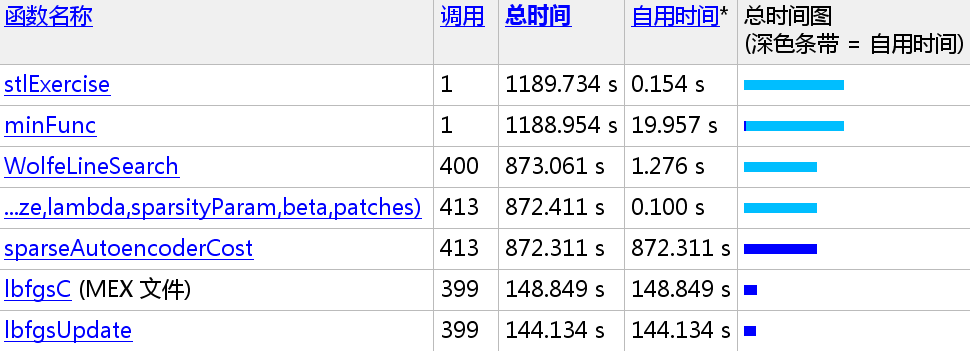
无监督学习训练 Sparse Autoencoder耗时较多:1189.734/60 = 19.8289 mins
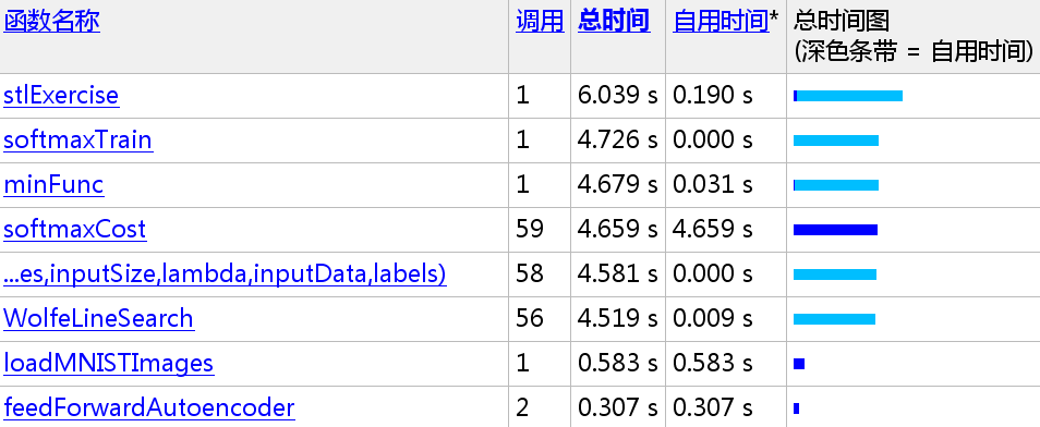
有监督的分类器学习较快,且没有完成100次迭代(56次)就完成了训练过程:
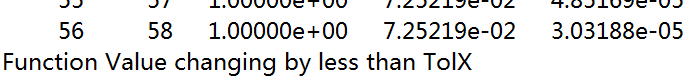
不过可能也因为这个原因,分类准确率比benchmark(98.3%)略低:98.221990%


 128
128

 被折叠的 条评论
为什么被折叠?
被折叠的 条评论
为什么被折叠?
 到【灌水乐园】发言


