Ubuntu16.04下使用tensorflow2.1 对fashion_mnist进行分类处理

使用TensorFlow2.0对fashion_mnist进行分类处理

环境主要还是在Ubuntu16.04,安装tensorflow2.0版本,数据集调用的是keras中的数据集.但是,在数据集的获取中,如果是在编写代码的过程中获取数据集,我自己的网络是不支持的,需要访问谷歌网站.所以我会先事先下载好fashion_mnist数据集,在/home目录下使用Ctrl+H打开隐藏文件夹找到.keras文件中的datasets,将下载好的数据集存放到文件夹中,从而来解决获取数据集失败的坑~~

# 导入相关的包
import tensorflow as tf
from tensorflow import keras
import numpy as np
import matplotlib.pyplot as plt

# 加载服装分类数据集
mnist = tf.keras.datasets.fashion_mnist

# 划分数据集(训练数据,测试数据)
(train_images,train_labels),(test_images,test_labels) = mnist.load_data()

# 服装类别标签
class_names = ['T-shirt/top', 'Trouser', 'Pullover', 'Dress', 'Coat',
               'Sandal', 'Shirt', 'Sneaker', 'Bag', 'Ankle boot']

# 训练图像的样本数量和图片尺寸
train_images.shape

# 测试图像标签数量
len(train_labels)

train_labels

test_images.shape

len(test_labels)

# 先查看训练数据的第一站图像
plt.figure()
plt.imshow(train_images[0])
plt.colorbar()
plt.grid()
plt.show()

# 对数据进行预处理,将数据的像素点划到0~1之间
train_images = train_images /255.0
test_images = test_images / 255.0

plt.figure(figsize=(10,10)) 
for i in range(25): #遍历25张图片
    plt.subplot(5,5,i+1) #分成5*5的长宽
    plt.xticks([]) #将横轴的数值取消
    plt.yticks([]) #将纵轴的数值取消
    plt.grid(False) #取消在图片上进行网格的描绘
    plt.imshow(train_images[i],cmap=plt.cm.binary) #输出图像,cmap=plt.cm.binary对颜色做出调整
    plt.xlabel(class_names[train_labels[i]]) #给每张图片打标签
plt.close

# 搭建网络
model = keras.Sequential([
#   对图像进行展平
    keras.layers.Flatten(input_shape=(28,28)),
#   128个神经元和使用relu的激活函数
    keras.layers.Dense(128,activation='relu'),
#   全连接层,使用softmax激活函数,将概率分布到10个类别中
    keras.layers.Dense(10,activation='softmax')
])

# 查看网络结构
model.summary()

第一个对图像进行展平的值是输入图像尺寸28*28 = 784
第二个 param的值是(输入的维度+1)*神经元= (784+1)*128=100480 之所以+1 是因为每个神经元都有一个偏置项bias
第3个:(128+1)*10= 1290

# 定义优化器,损失函数,指标
model.compile(optimizer = 'adam',
             loss=tf.keras.losses.sparse_categorical_crossentropy,
             metrics= ['accuracy'])

# 模型的训练,迭代次数
model.fit(train_images,train_labels,epochs= 5)

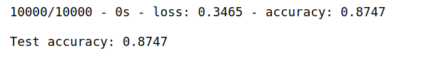
test_loss, test_acc = model.evaluate(test_images,  test_labels, verbose=2)

print('\nTest accuracy:', test_acc)

# 预测
probability_model= tf.keras.Sequential([model,tf.keras.layers.Softmax()])

predictions = probability_model.predict(test_images)

# 预测的结果分别代表了没中衣服的置信度
predictions[0]

np.argmax(predictions[0])

# 定义图像展示的函数
def plot_image(i,prediction_array,true_label,img):
        prediction_array = prediction_array
        true_label = true_label[i]
        img = img[i]
        plt.grid(False)
        plt.xticks([])
        plt.yticks([])

        plt.imshow(img,cmap=plt.cm.binary)

        prediction_label = np.argmax(prediction_array)
        if prediction_label == true_label:
            color = 'blue'
        else:
            color = 'red'
        plt.xlabel("{} {:2.0f}% ({})".format(class_names[prediction_label],
                                            100 * np.max(prediction_array),
                                            class_names[true_label]),
                                              color = color)

# 定义直方图
def plot_value_array(i,predicition_array,true_label):
    predicition_array= predicition_array
    true_label = true_label[i]
    
    plt.grid(False)
    plt.xticks(range(10))
    plt.yticks([])
    thisplot = plt.bar(range(10),predicition_array,color="#777777")
    plt.ylim([0,1])
    predicition_label = np.argmax(predicition_array)
    
    thisplot[predicition_label].set_color('red')
    thisplot[true_label].set_color('blue')

i = 0 
plt.figure(figsize=(6,3))
plt.subplot(1,2,1)
plot_image(i,predictions[i],test_labels,test_images)
plt.subplot(1,2,2)
plot_value_array(i,predictions[i],test_labels)
plt.show()

i = 12
plt.figure(figsize=(6,3))
plt.subplot(1,2,1)
plot_image(i, predictions[i], test_labels, test_images)
plt.subplot(1,2,2)
plot_value_array(i, predictions[i],  test_labels)
plt.show()

# 分批打印所以类别图片和概率值
num_rows = 5
num_cols = 3
num_images = num_rows * num_cols
plt.figure(figsize=(2*2*num_cols,2*num_rows))
for i in range(num_images):
    plt.subplot(num_rows,2*num_cols,2*i+1)
    plot_image(i, predictions[i], test_labels, test_images)
    plt.subplot(num_rows, 2*num_cols, 2*i+2)
    plot_value_array(i, predictions[i], test_labels)
    plt.tight_layout()
plt.show()