


Chapter 2.0 : Prerequisite 1 - Sufficient Statistics
PRML, OXford University Deep Learning Course, Machine Learning, Pattern Recognition
Christopher M. Bishop, PRML, Chapter 2 Probability Distributions
1. Introduction
In the process of estimating parameters, we summarize, or reduce, the information in a sample of size n ,
{X1,X2,...,Xn} , to a single number, such as the sample mean X¯ . The actual sample values are no longer important to us. That is, if we use a sample mean of 3 to estimate the population mean μ, it doesn’t matter if the original data values were(1,3,5) or (2,3,4) .
Problems:
- Has this process of reducing the
n
data points to a single number retained all of the information about
- Or has some information about the parameter been lost through the process of summarizing the data?
In this lesson, we’ll learn how to find statistics that summarize all of the information in a sample about the desired parameter. Such statistics are called sufficient statistics.
2. Definition of Sufficiency
2.1 Definition:
Let
- Why called “sufficient”?
- We say that
Y
is sufficient for
- Sufficiency means that if we know the value of
Y
, we cannot gain any further information about the parameter
2.2 Example 1 - Binomial Distribution:
Consider Bernoulli trials:
Let X1,X2,...,Xn be a random sample of n Bernoulli trials in which the success has the probability
p , and the fail with 1−p , i.e, P(Xi=1)=p , and P(Xi=0)=q=1−p , for i=1,2,...,n . Suppose, in a random sample of n=40 , that success events occur Y=∑ni=1Xi=22 in total. If we know the value of Y , the number of successes inn trials, can we gain any further information about the parameter p by considering other functions of the dataX1,X2,...,Xn ? Or equivalently is Y sufficient forp ?
Solution:
The definition of sufficiency tells us that if the conditional distribution of
X1,X2,...,Xn
, given the statistic
Y
, does not depend on
Now, for the sake of concreteness, suppose we were to observe a random sample of size n=3 in which x1=1,x2=0,x3=1 . In this case:
because (Y=1)≠(∑ni=1Xi=1+0+1=2) , corresponding to an impossible event in the numerator of (2.1) therefore with its probability being 0.
Now, let’s consider an event that is possible, namely
(X1=1,X2=0,X3=1,Y=2)
. In that case, we have, by independence:
So, in general:
and
Now, the denominator in (2.1) is the binomial probability of getting exactly
y
successes in
Putting the numerator and denominator together, we get
and
Conclusion 1:
We have just shown that the conditional distribution of
X1,X2,...,Xn
given
Y
does not depend on
3. Factorization Theorem
3.1 We need more easy method to identify sufficiency:
While the definition of sufficiency may make sense intuitively, it is not always all that easy to find the conditional distribution of
X1,X2,...,Xn given Y . Not to mention that we’d have to find the conditional distribution ofX1,X2,...,Xn given Y for everyY that we’d want to consider a possible sufficient statistic! Therefore, using the formal definition of sufficiency as a way of identifying a sufficient statistic for a parameter θ can often be a daunting road to follow. Thankfully, a theorem often referred to as the Factorization Theorem provides an easier alternative!
3.2 Factorization Theorem:
Let
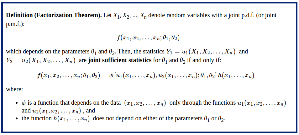
X1,X2,...,Xn denote random variables with joint probability density function or joint probability mass function f(x1,x2,...,xn∣θ) , which depends on the parameter θ . Then, the statistic Y=u(X1,X2,...,Xn) is sufficient for θ if and only if the p.d.f (or p.m.f.) can be factored into two components, that is:
f(x1,x2,...,xn∣θ)=ϕ[u(x1,x2,...,xn)∣θ]⋅h(x1,x2,...,xn)
where:
- ϕ is a function that depends on the data x1,x2,...,xn only through the function y=u(x1,x2,...,xn) , and
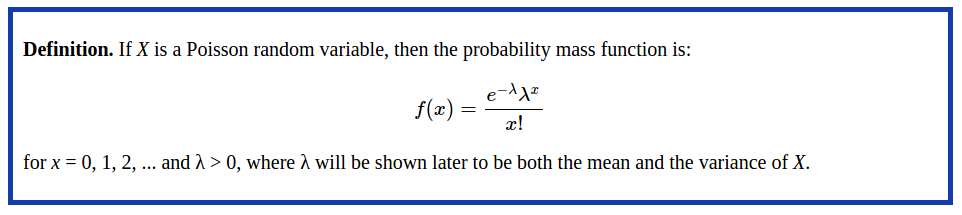
- the function h(x1,x2,...,xn) does not depend on the parameter θ .3.3 Example 2 - Poisson Distribution:
Recall that the mathematical constant e is the unique real number such that the value of the derivative (slope of the tangent line) of the function
f(x)=ex at the point x=0 is equal to 1 . It turns out that the constant is irrational, but to five decimal places, it equalse=2.71828 . Also, note that there are (theoretically) an infinite number of possible Poisson distributions. Any specific Poisson distribution depends on the parameter λ .Let X1,X2,...,Xn denote a random sample from a Poisson distribution with parameter λ>0 . Find a sufficient statistic for the parameter λ .
Solution:
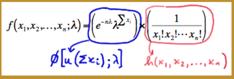
Because X1,X2,...,Xn is a random sample, the joint probability mass function of X1,X2,...,Xn is, by independence:
f(x1,x2,...,xn∣λ)=f(x1∣λ)⋅f(x2∣λ)⋅⋯⋅f(xn∣λ)=e−λλx1x1!⋅e−λλx2x2!⋅⋯⋅e−λλxnxn!=(e−nλλ∑xi)⋅(1x1!x2!…xn!)Hey, look at that! We just factored the joint p.m.f. into two functions, one ( ϕ ) being only a function of the statistic Y=∑ni=1Xi and the other ( h ) not depending on the parameter
λ :
We can also write the joint p.m.f. as:
f(x1,x2,...,xn∣λ)=(e−nλλnx¯)⋅(1x1!x2!…xn!)
Therefore, the Factorization Theorem tells us that Y=X¯ is also a sufficient statistic for λ .If you think about it, it makes sense that Y=X¯ and Y=∑ni=1Xi are both sufficient statistics, because if we know Y=X¯ , we can easily find Y=∑ni=1Xi , and vice verse.
Conclusion 2:
There can be more than one sufficient statistic for a parameter θ . In general, if Y is a sufficient statistic for a parameter
θ , then every one-to-one function of Y not involvingθ is also a sufficient statistic for θ .3.4 Example 3 - Gaussian Distribution N(μ,1) :
Let X1,X2,...,Xn be a random sample from a normal distribution with mean μ and variance σ=1 . Find a sufficient statistic for the parameter μ .
Solution:
For i.i.d. data X1,X2,...,Xn , the joint probability density function of X1,X2,...,Xn is
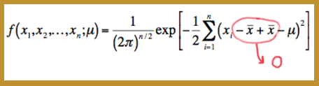
f(x1,x2,...,xn∣μ)=f(x1∣μ)×f(x2∣μ)×⋯×f(xn∣μ)=1(2π)1/2exp[−12(x1−μ)2]×1(2π)1/2exp[−12(x2−μ)2]×⋯×1(2π)1/2exp[−12(xn−μ)2]=1(2π)n/2exp[−12∑i=1n(xi−μ)2]A trick to making the factoring of the joint p.d.f. an easier task is to add 0 to the quantity in parentheses in the summation. That is:
Now, squaring the quantity in parentheses, we get:
f(x1,x2,...,xn;μ)=1(2π)n/2exp[−12∑i=1n[(xi−x¯)2+2(xi−x¯)(x¯−μ)+(x¯−μ)2]]
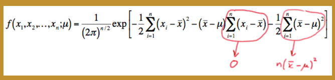
And then distributing the summation, we get:
f(x1,x2,...,xn;μ)=1(2π)n/2exp[−12∑i=1n(xi−x¯)2−(x¯−μ)∑i=1n(xi−x¯)−12∑i=1n(x¯−μ)2]But, the middle term in the exponent is 0 , and the last term, because it doesn’t depend on the index
i , can be added up n times:
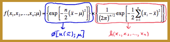
So, simplifying, we get:
f(x1,x2,...,xn;μ)={exp[−n2(x¯−μ)2]}×{1(2π)n/2exp[−12∑i=1n(xi−x¯)2]} In summary, we have factored the joint p.d.f. into two functions, one ( ϕ ) being only a function of the statistic Y=X¯ and the other ( h ) not depending on the parameter
μ :
Conclusion 3:
- Therefore, the Factorization Theorem tells us that Y=X¯=1n∑ni=1Xi is a sufficient statistic for μ .
- Now, Y=X¯3 is also sufficient for μ , because if we are given the value of X¯3 , we can easily get the value of X¯ through the one-to-one function w=y1/3 , that is W=(X¯3)1/3=X¯ .
- However, Y=X¯2 is not a sufficient statistic for μ , because it is not a one-to-one function, with both +X¯ and −X¯ mapped to X¯2 .
3.5 Example 4 - Exponential Distribution:
Let X1,X2,...,Xn be a random sample from an exponential distribution with parameter θ . Find a sufficient statistic for the parameter θ .
Solution:
The joint probability density function of X1,X2,...,Xn is, by independence:
f(x1,x2,...,xn;θ)=f(x1;θ)×f(x2;θ)×...×f(xn;θ)
the joint p.d.f. is:
f(x1,x2,...,xn;θ)=1θexp(−x1θ)×1θexp(−x2θ)×...×1θexp(−xnθ)
Now, simplifying, by adding up all n of theθs′ and the nxi ’s in the exponents, we get:
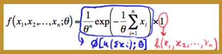
f(x1,x2,...,xn;θ)=1θnexp(−1θ∑i=1nxi)
We have again factored the joint p.d.f. into two functions, one ( ϕ ) being only a function of the statistic Y=∑ni=1Xi and the other ( h=1 ) not depending on the parameter θ :
Conclusion 4:
Therefore, the Factorization Theorem tells us that Y=∑ni=1Xi is a sufficient statistic for θ . And, since Y=X¯ is a one-to-one function of Y=∑ni=1Xi , it implies that Y=X¯ is also a sufficient statistic for θ .
4. Exponential Form
4.1 Exponential Form
You might not have noticed that in all of the examples we have considered so far in this lesson, every p.d.f. or p.m.f. could be written in what is often called exponential form, that is:
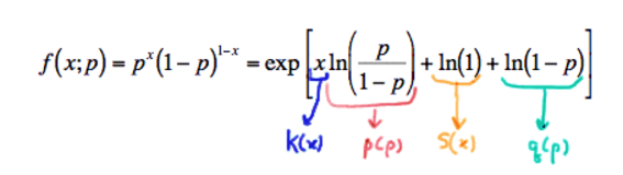
f(x∣θ)=exp[K(x)p(θ)+S(x)+q(θ)]1) Exponential Form of Bernoulli Distribution:
For example, the Bernoulli random variables with p.m.f. is written in exponential form as:
with
- (1) K(x)=x and S(x)=ln(1) being functions only of x ,
- (2)
p(p)=lnp1−p and q(p)=ln(1−p) being functions only of the parameter p , and- (3) the support
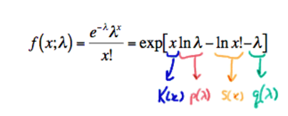
x=0,1 not depending on the parameter p .2) Exponential Form of Poisson Distribution:
with
- (1)
K(x)=x and S(x)=−ln(x!) being functions only of x ,- (2)
p(λ)=lnλ and q(λ)=−λ being functions only of the parameter λ , and- (3) the support x=0,1,2,… not depending on the parameter λ .
3) Exponential Form of Gaussian Distribution N(μ,1) :
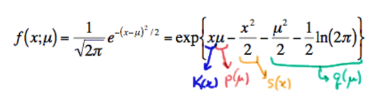
with
- (1) K(x)=x and S(x)=−x22 being functions only of x ,
- (2)
p(μ)=μ and q(μ)=−μ22−12ln(2π) being functions only of the parameter μ , and- (3) the support −∞<x<∞ not depending on the parameter μ .
4) Exponential Form of Exponential Distribution:
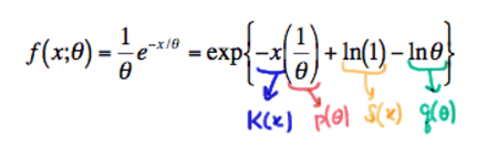
with
- (1) K(x)=−x and S(x)=ln(1)=0 being functions only of x ,
- (2)
p(θ)=1θ and q(θ)=−lnθ being functions only of the parameter θ , and- (3) the support x≥0 not depending on the parameter θ .
4.2 Exponential Criterion
It turns out that writing p.d.f.s and p.m.f.s in exponential form provides us yet a third way of identifying sufficient statistics for our parameters. The following theorem tells us how.
Theorem:
Let X1,X2,...,Xn be a random sample from a distribution with a p.d.f. or p.m.f. of the exponential form:
f(x∣θ)=exp[K(x)p(θ)+S(x)+q(θ)]
with a support that does not depend on θ, that is,
- (1) K(x) and S(x)= being functions only of x ,
- (2)p(θ) and q(θ) being functions only of the parameter θ , and
- (3) the support being free of the parameter θ .Then, the statistic:
∑i=1nK(Xi)is sufficient for θ .Proof:
f(x1,x2,...,xn;θ)=f(x1;θ)×f(x2;θ)×...×f(xn;θ)
f(x1,...,xn;θ)=exp[K(x1)p(θ)+S(x1)+q(θ)]×...×exp[K(xn)p(θ)+S(xn)+q(θ)]
Collecting like terms in the exponents, we get:f(x1,...,xn;θ)=exp[p(θ)∑i=1nK(xi)+∑i=1nS(xi)+nq(θ)]
which can be factored as:f(x1,...,xn;θ)={exp[p(θ)∑i=1nK(xi)+nq(θ)]}×{exp[∑i=1nS(xi)]}
We have factored the joint p.m.f. or p.d.f. into two functions:
- one ( ϕ ) being only a function of the statistic Y=∑ni=1K(Xi) and
- the other ( h ) not depending on the parameterθ :
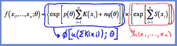
Therefore, the Factorization Theorem tells us that Y=∑ni=1K(Xi) is a sufficient statistic for θ .
4.3 Example 5 - Geometric Distribution:
Let X1,X2,...,Xn be a random sample from a geometric distribution with parameter p . Find a sufficient statistic for the parameter
p .Solution:
The probability mass function of a geometric random variable is:
f(x;p)=(1−p)x−1pfor x=1,2,3,… The p.m.f. can be written in exponential form as
f(x;p)=exp[xlog(1−p)+log(1)+log(p1−p)]Conclusion 5:
Therefore, Y=∑ni=1Xi is sufficient for p . Easy as pie!
5. Two or More Parameters
What happens if a probability distribution has two parameters,
θ1 and θ2 , say, for which we want to find sufficient statistics, Y1 and Y2 ? Fortunately, the definitions of sufficiency can easily be extended to accommodate two (or more) parameters. Let’s start by extending the Factorization Theorem.5.1 Factorization Theorem
5.2 Example 6 - Gaussian Distribution N(μ,σ2) :
Let X1,X2,...,Xn denote a random sample from a normal distribution N(θ1,θ1) . That is, θ1 denotes the mean μ and θ2 denotes the variance σ2 . Use the Factorization Theorem to find joint sufficient statistics for θ1 and θ2 .
Solution:
The joint probability density function of X1,X2,...,Xn is, by independence:
f(x1,x2,...,xn;θ1,θ2)=f(x1;θ1,θ2)×f(x2;θ1,θ2)×...×f(xn;θ1,θ2)Due to the Gaussian pdf
f(xi∣θ1,θ2)=1(2πθ2)1/2exp[−12(xi−θ1)2θ2]We get
f(x1,x2,...,xn;θ1,θ2)=(12πθ2−−−−√)nexp[−12∑ni=1(xi−θ1)2θ2]
Rewriting the first factor, and squaring the quantity in parentheses, and distributing the summation, in the second factor, we get:f(x1,x2,...,xn;θ1,θ2)=exp⎡⎣log(12πθ2−−−−√)n⎤⎦exp[−12θ2{∑i=1nx2i−2θ1∑i=1nxi+∑i=1nθ21}]Simplifying yet more, we get:
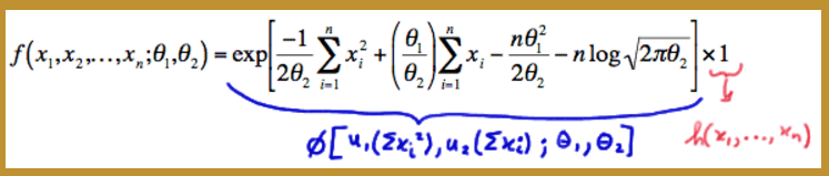
f(x1,x2,...,xn;θ1,θ2)=exp[−12θ2∑i=1nx2i+θ1θ2∑i=1nxi−nθ212θ2−nlog2πθ2−−−−√]Look at that! We have factored the joint p.d.f. into two functions, one ( ϕ ) being only a function of the statistic Y1=∑ni=1X2i and Y2=∑ni=1Xi , and the other ( h=1 ) not depending on the parameter θ1 and θ2 :
Conclusion 6.1:
- Therefore, the Factorization Theorem tells us that Y1=∑ni=1X2i and Y2=∑ni=1Xi are joint sufficient statistics for θ1 and θ2 .
- And, the one-to-one functions of Y1 and Y2 , namely:
X¯=Y2n=1n∑i=1nXi
andS2=Y1−(Y22/n)n−1=1n−1[∑i=1nX2i−nX¯2]are also joint sufficient statistics for θ1 and θ2 .- We have just shown that the intuitive estimators of μ and σ2 are also sufficient estimators. That is, the data contain no more information than the estimators X¯ and S2 do about the parameters μ and σ2 . That seems like a good thing!
5.3 Exponential Criterion
We have just extended the Factorization Theorem. Now, the Exponential Criterion can also be extended to accommodate two (or more) parameters. It is stated here without proof.
Exponential Criterion:
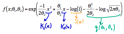
Let X1,X2,...,Xn be a random sample from a distribution with a p.d.f. or p.m.f. of the exponential form: f(x;θ1,θ2)=exp[K1(x)p1(θ1,θ2)+K2(x)p2(θ1,θ2)+S(x)+q(θ1,θ2)]with a support that does not depend on the parameters θ1 and θ2 . Then, the statistics Y1=∑ni=1K1(Xi) and Y2=∑ni=1K2(Xi) are jointly sufficient for θ1 and θ2 .5.4 Example 6 - Gaussian Distribution N(μ,σ2) (continued):
Let X1,X2,...,Xn denote a random sample from a normal distribution N(θ1,θ1) . That is, θ1 denotes the mean μ and θ2 denotes the variance σ2 . Use the Exponential Criterion to find joint sufficient statistics for θ1 and θ2 .
Solution:
The probability density function of a normal random variable with mean θ1 and variance θ2 can be written in exponential form as:
Conclusion 6.2:
Therefore, the statistics Y1=∑ni=1X2i and Y2=∑ni=1Xi are joint sufficient statistics for θ1 and θ2 .
6. Reference
[1]: Lesson 53: Sufficient Statistics (ttps://onlinecourses.science.psu.edu/stat414/print/book/export/html/244)


 945
945

 被折叠的 条评论
为什么被折叠?
被折叠的 条评论
为什么被折叠?
 到【灌水乐园】发言


