


本讲我们将会创建一个合成特征,即另外两个特征的比例,将此新特征用作线性回归模型的输入,并通过识别和截取(移除)输入数据中的离群值来提高模型的有效性。
以下代码摘自谷歌的官方示例。
还是用回之前的房价数据
from __future__ import print_function

import math

from IPython import display
from matplotlib import cm
from matplotlib import gridspec
import matplotlib.pyplot as plt
import numpy as np
import pandas as pd
import sklearn.metrics as metrics
import tensorflow as tf
from tensorflow.python.data import Dataset

tf.logging.set_verbosity(tf.logging.ERROR)
pd.options.display.max_rows = 10
pd.options.display.float_format = '{:.1f}'.format

california_housing_dataframe = pd.read_csv("https://download.mlcc.google.cn/mledu-datasets/california_housing_train.csv", sep=",")

california_housing_dataframe = california_housing_dataframe.reindex(
    np.random.permutation(california_housing_dataframe.index))
california_housing_dataframe["median_house_value"] /= 1000.0
california_housing_dataframe
设置输入函数,并针对模型训练来定义该函数
def my_input_fn(features, targets, batch_size=1, shuffle=True, num_epochs=None):
    """训练单个批次的特征的线性回归模型

    Args:
      features: 特征
      targets: 标签(目标)
      batch_size: 要传递给模型的批次大小
      shuffle: 是否随机处理
      num_epochs: 重复次数. None = 无限次重复
    Returns:
      下一批次的特征和标签的元组
    """

    # 将pandas数据转换为np数组的dict
    features = {key:np.array(value) for key,value in dict(features).items()}

    # 构建数据集,并配置批处理的重复次数
    ds = Dataset.from_tensor_slices((features,targets)) # 最多2GB
    ds = ds.batch(batch_size).repeat(num_epochs)

    # 看看是否要随机数据
    if shuffle:
      ds = ds.shuffle(buffer_size=10000)

    # 返回下一批次的特征和标签
    features, labels = ds.make_one_shot_iterator().get_next()
    return features, labels
建模代码
def train_model(learning_rate, steps, batch_size, input_feature="total_rooms"):
  """训练线性回归模型

  Args:
    learning_rate: 学习率
    steps: 训练步骤的总数。 训练步骤包括使用单个批次的前向和后向传递
    batch_size: 批量大小
    input_feature: `california_housing_dataframe`的特征列
  """

  periods = 10
  steps_per_period = steps / periods

  my_feature = input_feature
  my_feature_data = california_housing_dataframe[[my_feature]]
  my_label = "median_house_value"
  targets = california_housing_dataframe[my_label]

  # 创建特征列
  feature_columns = [tf.feature_column.numeric_column(my_feature)]

  training_input_fn = lambda:my_input_fn(my_feature_data, targets, batch_size=batch_size)
  prediction_input_fn = lambda: my_input_fn(my_feature_data, targets, num_epochs=1, shuffle=False)

  # 创建线性回归模型
  my_optimizer = tf.train.GradientDescentOptimizer(learning_rate=learning_rate)
  my_optimizer = tf.contrib.estimator.clip_gradients_by_norm(my_optimizer, 5.0)
  linear_regressor = tf.estimator.LinearRegressor(
      feature_columns=feature_columns,
      optimizer=my_optimizer
  )

  # 绘制每个时期模型行的状态
  plt.figure(figsize=(15, 6))
  plt.subplot(1, 2, 1)
  plt.title("Learned Line by Period")
  plt.ylabel(my_label)
  plt.xlabel(my_feature)
  sample = california_housing_dataframe.sample(n=300)
  plt.scatter(sample[my_feature], sample[my_label])
  colors = [cm.coolwarm(x) for x in np.linspace(-1, 1, periods)]

  # 在循环内训练模型,以便定期评估损失指标
  print("Training model...")
  print("RMSE (on training data):")
  root_mean_squared_errors = []
  for period in range (0, periods):
    # 训练模型
    linear_regressor.train(
        input_fn=training_input_fn,
        steps=steps_per_period
    )
    # 计算预测
    predictions = linear_regressor.predict(input_fn=prediction_input_fn)
    predictions = np.array([item['predictions'][0] for item in predictions])

    # 计算损失
    root_mean_squared_error = math.sqrt(
        metrics.mean_squared_error(predictions, targets))
    # 偶尔打印一下当前的损失
    print("  period %02d : %0.2f" % (period, root_mean_squared_error))
    # 将损失指标加到root_mean_squared_errors中
    root_mean_squared_errors.append(root_mean_squared_error)
    # 跟踪一下 weights 和 biases 随时间的变化
    # 应用一些数学运算来确保数据和线条可以整齐地绘制
    y_extents = np.array([0, sample[my_label].max()])

    weight = linear_regressor.get_variable_value('linear/linear_model/%s/weights' % input_feature)[0]
    bias = linear_regressor.get_variable_value('linear/linear_model/bias_weights')

    x_extents = (y_extents - bias) / weight
    x_extents = np.maximum(np.minimum(x_extents,
                                      sample[my_feature].max()),
                           sample[my_feature].min())
    y_extents = weight * x_extents + bias
    plt.plot(x_extents, y_extents, color=colors[period])
  print("Model training finished.")

  # 输出一段时间内的损失指标图表
  plt.subplot(1, 2, 2)
  plt.ylabel('RMSE')
  plt.xlabel('Periods')
  plt.title("Root Mean Squared Error vs. Periods")
  plt.tight_layout()
  plt.plot(root_mean_squared_errors)

  # 输出包含校准数据的表格
  calibration_data = pd.DataFrame()
  calibration_data["predictions"] = pd.Series(predictions)
  calibration_data["targets"] = pd.Series(targets)
  display.display(calibration_data.describe())

  print("Final RMSE (on training data): %0.2f" % root_mean_squared_error)
  return calibration_data
合成特征
total_rooms 和 population 特征都会统计指定街区的相关总计数据。
但是,如果一个街区比另一个街区的人口更密集,会怎么样?我们可以创建一个合成特征(即 total_rooms 与 population 的比例)来探索街区人口密度与房屋价值中位数之间的关系。
california_housing_dataframe["rooms_per_person"] = (
    california_housing_dataframe["total_rooms"] / california_housing_dataframe["population"])

calibration_data = train_model(
    learning_rate=0.05,
    steps=500,
    batch_size=5,
    input_feature="rooms_per_person")
识别离群值
我们可以通过创建预测值与目标值的散点图来可视化模型效果。理想情况下,这些值将位于一条完全相关的对角线上。
使用我们刚刚训练过的人均房间数模型,并使用 Pyplot 的 scatter() 创建预测值与目标值的散点图。看看是否有异常情况。
plt.figure(figsize=(15, 6))
plt.subplot(1, 2, 1)
plt.scatter(calibration_data["predictions"], calibration_data["targets"])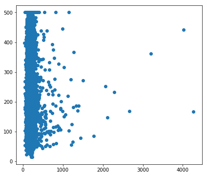
校准数据显示,大多数散点与一条线对齐。这条线几乎是垂直的,我们稍后再讲解。现在,我们重点关注偏离这条线的点。我们注意到这些点的数量相对较少。
如果我们绘制 rooms_per_person 的直方图,则会发现我们的输入数据中有少量离群值:
plt.subplot(1, 2, 2)
_ = california_housing_dataframe["rooms_per_person"].hist()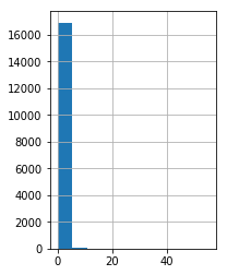
截取离群值
从前面创建的直方图显示,大多数值都小于 5。我们将 rooms_per_person 的值截取为 5,然后绘制直方图以再次检查结果。
california_housing_dataframe["rooms_per_person"] = (
    california_housing_dataframe["rooms_per_person"]).apply(lambda x: min(x, 5))

_ = california_housing_dataframe["rooms_per_person"].hist()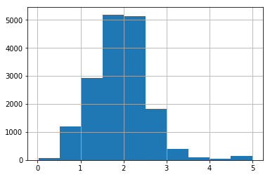
为了验证截取是否有效,我们再训练一次模型,并输出校准数据
calibration_data = train_model(
    learning_rate=0.05,
    steps=500,
    batch_size=5,
    input_feature="rooms_per_person")

_ = plt.scatter(calibration_data["predictions"], calibration_data["targets"])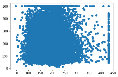
这个就是我跑出来的结果,有兴趣的可以自行去尝试一下。


 被折叠的 条评论
为什么被折叠?
被折叠的 条评论
为什么被折叠?
 到【灌水乐园】发言


