import numpy as np
import pandas as pd
from wordcloud import WordCloud
from textblob import TextBlob
import matplotlib.pyplot as plt
from collections import Counter
from nltk.corpus import stopwords
import string
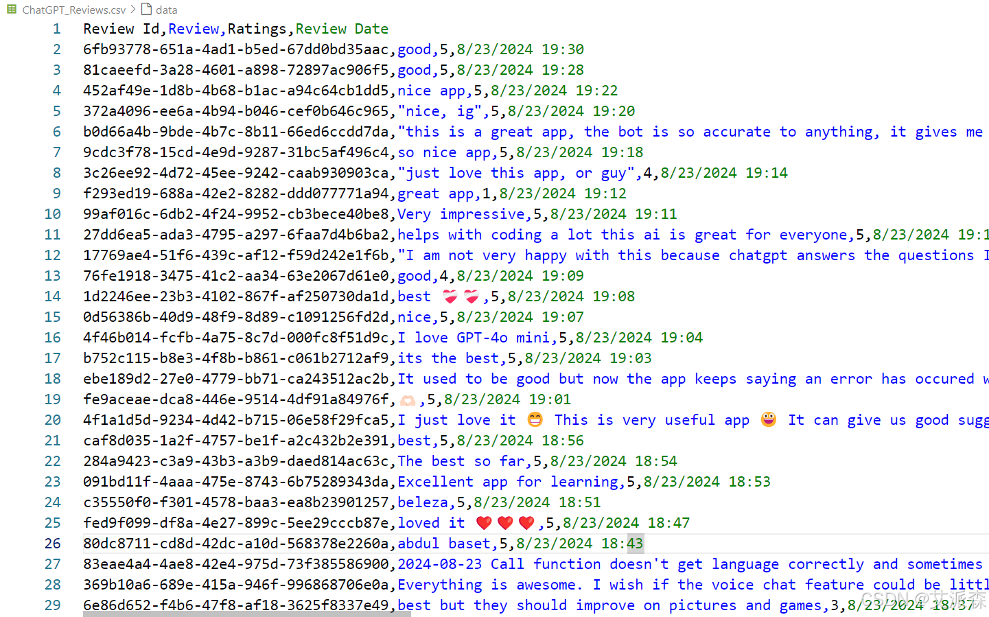
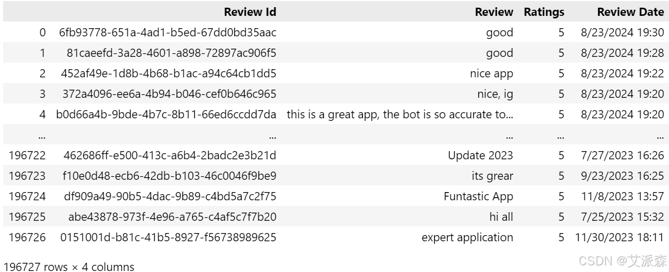
df = pd.read_csv('ChatGPT_Reviews.csv')
df
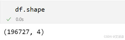
df.shape
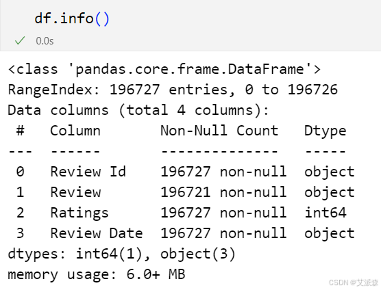
df.info()
# 将评论日期转为日期类型,无法转换的异常数据设置为空值
df['Review Date'] = pd.to_datetime(df['Review Date'], errors='coerce')
# 将评分转为数值类型,无法转换的异常数据设置为空值
df['Ratings'] = pd.to_numeric(df['Ratings'], errors='coerce')
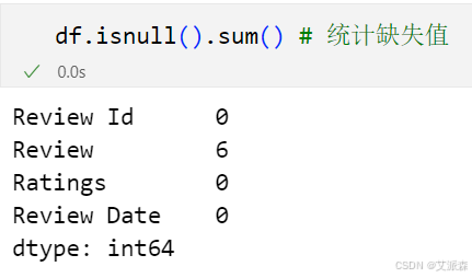
df.isnull().sum() # 统计缺失值
df.dropna(inplace=True) # 删除缺失值
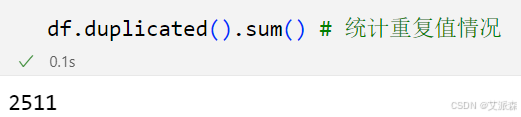
df.duplicated().sum() # 统计重复值情况
df.drop_duplicates(inplace=True) # 删除重复值
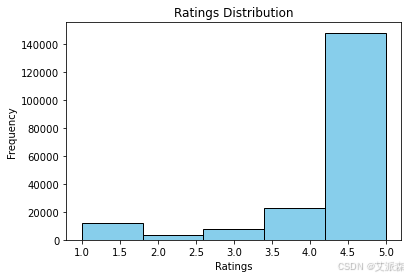
# 评分分布
def plot_ratings_distribution(df):
    plt.hist(df['Ratings'], bins=5, edgecolor='black', color='skyblue')
    plt.title("Ratings Distribution")
    plt.xlabel("Ratings")
    plt.ylabel("Frequency")
    plt.show()

plot_ratings_distribution(df)
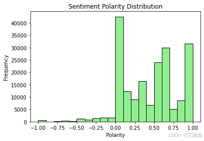
# 对评论进行情感分析
def analyze_sentiments(df):
    def analyze_sentiment(text):
        analysis = TextBlob(text)
        return analysis.polarity

    df['Sentiment'] = df['Review'].apply(analyze_sentiment)
    plt.hist(df['Sentiment'], bins=20, color='lightgreen', edgecolor='black')
    plt.title("Sentiment Polarity Distribution")
    plt.xlabel("Polarity")
    plt.ylabel("Frequency")
    plt.show()
    return df

analyze_sentiments(df)
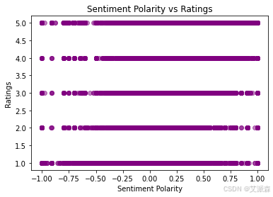
# 情绪极性与评级的散点图
def plot_sentiment_vs_ratings(df):
    plt.scatter(df['Sentiment'], df['Ratings'], alpha=0.5, color='purple')
    plt.title("Sentiment Polarity vs Ratings")
    plt.xlabel("Sentiment Polarity")
    plt.ylabel("Ratings")
    plt.show()

plot_sentiment_vs_ratings(df)
# 生成并显示评论的词云
def generate_word_cloud(df):
    text = " ".join(review for review in df['Review'])
    wordcloud = WordCloud(width=800, height=400, background_color='white').generate(text)
    plt.figure(figsize=(10, 5))
    plt.imshow(wordcloud, interpolation='bilinear')
    plt.axis("off")
    plt.show()

generate_word_cloud(df)
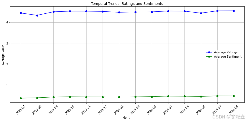
# 分析评级和情绪的时间趋势
def temporal_trends(df):
    df['Review Month'] = df['Review Date'].dt.to_period('M')
    monthly_avg_ratings = df.groupby('Review Month')['Ratings'].mean()
    monthly_avg_sentiment = df.groupby('Review Month')['Sentiment'].mean()

    months = monthly_avg_ratings.index.astype(str)

    plt.figure(figsize=(12, 6))
    plt.plot(months, monthly_avg_ratings, label='Average Ratings', marker='o', color='blue')
    plt.plot(months, monthly_avg_sentiment, label='Average Sentiment', marker='o', color='green')
    plt.title("Temporal Trends: Ratings and Sentiments")
    plt.xlabel("Month")
    plt.ylabel("Average Value")
    plt.legend()
    plt.grid()
    plt.xticks(rotation=45)
    plt.tight_layout()
    plt.show()

temporal_trends(df)
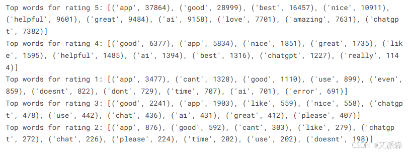
def get_top_words(reviews, n=10):
    stop_words = set(stopwords.words('english'))
    words = " ".join(reviews).lower().translate(str.maketrans('', '', string.punctuation)).split()
    words = [word for word in words if word not in stop_words]
    return Counter(words).most_common(n)

for rating in df['Ratings'].unique():
    top_words = get_top_words(df[df['Ratings'] == rating]['Review'], n=10)
    print(f"Top words for rating {rating}: {top_words}")
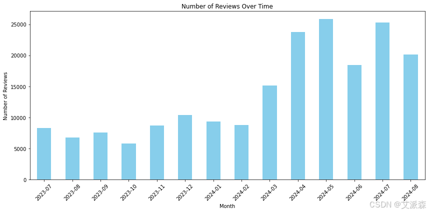
# 临时评论计数趋势分析一段时间内提交的评论数量,以确定高用户活动的时期
review_counts = df.groupby(df['Review Date'].dt.to_period('M')).size()
review_counts.plot(kind='bar', color='skyblue', figsize=(12, 6))
plt.title("Number of Reviews Over Time")
plt.xlabel("Month")
plt.ylabel("Number of Reviews")
plt.xticks(rotation=45)
plt.tight_layout()
plt.show()
import seaborn as sns
def categorize_sentiment(polarity):
if polarity > 0.2:
return "Positive"
elif polarity < -0.2:
return "Negative"
else:
return "Neutral"
if 'Sentiment' in df.columns:
df['Sentiment Category'] = df['Sentiment'].apply(categorize_sentiment)
else:
print("Error: 'Sentiment' column not found. Ensure sentiment analysis has been performed.")
print(df.columns)
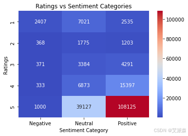
heatmap_data = df.pivot_table(index='Ratings', columns='Sentiment Category', aggfunc='size', fill_value=0)
sns.heatmap(heatmap_data, annot=True, fmt='d', cmap='coolwarm')
plt.title("Ratings vs Sentiment Categories")
plt.xlabel("Sentiment Category")
plt.ylabel("Ratings")
plt.show()
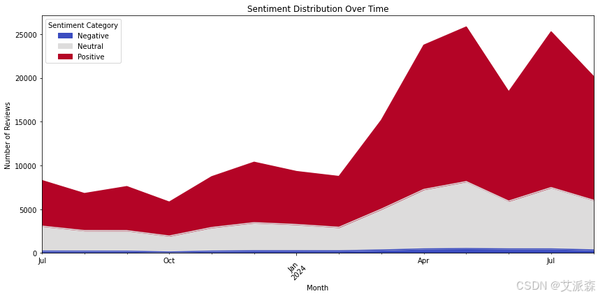
# 不同时期的情感变化趋势
sentiment_trend = df.groupby([df['Review Date'].dt.to_period('M'), 'Sentiment Category']).size().unstack(fill_value=0)
sentiment_trend.plot(kind='area', stacked=True, figsize=(12, 6), colormap='coolwarm')
plt.title("Sentiment Distribution Over Time")
plt.xlabel("Month")
plt.ylabel("Number of Reviews")
plt.legend(title="Sentiment Category")
plt.xticks(rotation=45)
plt.tight_layout()
plt.show()
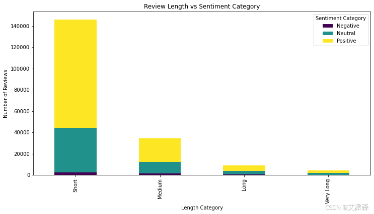
# 分析不同长度评论的情感
df['Review Length'] = df['Review'].str.len()
df['Length Category'] = pd.cut(df['Review Length'],
                               bins=[0, 50, 150, 300, 1000],
                               labels=['Short', 'Medium', 'Long', 'Very Long'])
length_sentiment = pd.crosstab(df['Length Category'], df['Sentiment Category'])
length_sentiment.plot(kind='bar', stacked=True, figsize=(12, 6), colormap='viridis')
plt.title("Review Length vs Sentiment Category")
plt.xlabel("Length Category")
plt.ylabel("Number of Reviews")
plt.legend(title="Sentiment Category")
plt.show()
- 1.
- 2.
- 3.
- 4.
- 5.
- 6.
- 7.
- 8.
- 9.
- 10.
- 11.
- 12.
- 13.
- 14.
- 15.
- 16.
- 17.
- 18.
- 19.
- 20.
- 21.
- 22.
- 23.
- 24.
- 25.
- 26.
- 27.
- 28.
- 29.
- 30.
- 31.
- 32.
- 33.
- 34.
- 35.
- 36.
- 37.
- 38.
- 39.
- 40.
- 41.
- 42.
- 43.
- 44.
- 45.
- 46.
- 47.
- 48.
- 49.
- 50.
- 51.
- 52.
- 53.
- 54.
- 55.
- 56.
- 57.
- 58.
- 59.
- 60.
- 61.
- 62.
- 63.
- 64.
- 65.
- 66.
- 67.
- 68.
- 69.
- 70.
- 71.
- 72.
- 73.
- 74.
- 75.
- 76.
- 77.
- 78.
- 79.
- 80.
- 81.
- 82.
- 83.
- 84.
- 85.
- 86.
- 87.
- 88.
- 89.
- 90.
- 91.
- 92.
- 93.
- 94.
- 95.
- 96.
- 97.
- 98.
- 99.
- 100.
- 101.
- 102.
- 103.
- 104.
- 105.
- 106.
- 107.
- 108.
- 109.
- 110.
- 111.
- 112.
- 113.
- 114.
- 115.
- 116.
- 117.
- 118.
- 119.
- 120.
- 121.
- 122.
- 123.
- 124.
- 125.
- 126.
- 127.
- 128.
- 129.
- 130.
- 131.
- 132.
- 133.
- 134.
- 135.
- 136.
- 137.
- 138.
- 139.
- 140.
- 141.
- 142.
- 143.
- 144.
- 145.
- 146.


 被折叠的 条评论
为什么被折叠?
被折叠的 条评论
为什么被折叠?
 到【灌水乐园】发言


