【论文伴读】【TimeSformer】Is Space-Time Attention All You Need for Video Understanding?-Part2

前言

论文题目：Is Space-Time Attention All You Need for Video Understanding?
论文链接：https://arxiv.org/pdf/2102.05095.pdf
github 地址：https://github.com/lucidrains/TimeSformer-pytorch

3. The TimeSformer Model

段落1：

原文：“Input clip. The TimeSformer takes as input a clip $X\in {\mathbb{R}}^{H\times W\times 3\times F}$ consisting of F RGB frames of size H × W sampled from the original video.”
翻译：输入片段。TimeSformer接收输入片段$X\in {\mathbb{R}}^{H\times W\times 3\times F}$，其中包含从原始视频中采样的F帧H × W大小的RGB帧。
解释：
重点词汇：
clip：视频片段
RGB frames：RGB帧
数学表示：使用张量表示输入数据
明确输入数据格式和维度

段落2-3：

原文：“Decomposition into patches. Following the ViT (Dosovitskiy et al., 2020), we decompose each frame into N non-overlapping patches, each of size P × P, such that the N patches span the entire frame, i.e., N = HW/P2. We flatten these patches into vectors x(p,t) ∈ R3P2 with p = 1, . . . , N denoting spatial locations and t = 1, . . . , F depicting an index over frames.”
翻译：分解为图像块。遵循ViT的方法，我们将每一帧分解为N个不重叠的图像块，每个大小为P × P，使得N个图像块覆盖整个帧，即$N=\frac{HW}{P^2}$。我们将这些图像块展平为向量$\mathbf{x}(p,t)\in {\mathbb{R}}^{3P^2}$，其中p = 1, . . . , N表示空间位置，t = 1, . . . , F表示帧的索引。
解释：
重点词汇：
non-overlapping patches：不重叠的图像块
flatten：展平
详细说明数据预处理步骤
建立空间和时间索引系统

B. 段落整体理解

段落主旨：详细说明TimeSformer模型的输入处理方式
核心要点：
输入数据格式定义
图像块分解方法
向量化处理
索引系统设计
C. 专业知识拓展

术语解释：
RGB frames：由红、绿、蓝三个通道组成的图像帧
patches：将图像分割成的小块区域
flattening：将多维数据转换为一维向量的过程
spatial locations：空间位置，指图像中的位置坐标

句子1：

原文：“We linearly map each patch x(p,t) into an embedding vector $z_{(p,t)}^{(0)}\in {\mathbb{R}}^D$ by means of a learnable matrix $E\in {\mathbb{R}}^{D\times 3P^2}$:”

翻译：我们通过可学习矩阵$E\in {\mathbb{R}}^{D\times 3P^2}$将每个图像块x(p,t)线性映射为嵌入向量$z_{(p,t)}^{(0)}\in {\mathbb{R}}^D$：

句子2：

原文：“where $e_{(p,t)}^{pos}\in {\mathbb{R}}^D$ represents a learnable positional embedding added to encode the spatiotemporal position of each patch.”
翻译：其中$e_{(p,t)}^{pos}\in {\mathbb{R}}^D$表示一个可学习的位置嵌入，用于编码每个图像块的时空位置。
解释：
数学表示：
$e_{(p,t)}^{pos}\in {\mathbb{R}}^D$
强调位置嵌入的可学习性
说明时空编码的作用

句子3：

原文：“The resulting sequence of embedding vectors z(0)(p,t) for p = 1, . . . , N, and t = 1, . . . , F represents the input to the Transformer, and plays a role similar to the sequences of embedded words that are fed to text Transformers in NLP.”
翻译：生成的嵌入向量序列z(0)(p,t)（其中p = 1, . . . , N，t = 1, . . . , F）作为Transformer的输入，其作用类似于NLP中输入到文本Transformer的词嵌入序列。
解释：
建立与NLP的类比
说明序列处理的相似性

句子4：

原文：“As in the original BERT Transformer (Devlin et al., 2018), we add in the first position of the sequence a special learnable vector z(0)(0,0) ∈ RD representing the embedding of the classification token.”
翻译：与原始BERT Transformer一样，我们在序列的第一个位置添加一个特殊的可学习向量$z_{(0,0)}^{(0)}\in {\mathbb{R}}^D$，代表分类标记的嵌入。

解释：
借鉴BERT的设计思想
用于后续分类任务

B. 段落整体理解

段落主旨：详细说明位置编码和分类标记的实现方式
核心要点：
位置嵌入的设计
与NLP模型的对应关系
分类标记的引入
序列处理的架构

C. 专业知识拓展

术语解释：
位置嵌入：用于保留序列中元素位置信息的编码方式
时空位置：同时包含空间和时间维度的位置信息
BERT：一种先进的自然语言处理模型
分类标记：用于整体特征表示的特殊向量

段落1：

原文：“Our Transformer consists of L encoding blocks. At each block $\ell$, a query/key/value vector is computed for each patch from the representation ${\mathbf{z}}_{(p,t)}^{(\ell -1)}$ encoded by the preceding block:”
翻译：我们的Transformer由L个编码块组成。在每个块$\ell$中，从前一个块编码的表示${\mathbf{z}}_{(p,t)}^{(\ell -1)}$ 为每个图像块计算query/key/value向量：

三个公式：
$${\mathbf{q}}_{(p,t)}^{(\ell ,a)}=W^{(Q_{\ell ,a})}\text{LN}({\mathbf{z}}_{(p,t)}^{(\ell -1)})\in {\mathbb{R}}^{D_h}$$
$${\mathbf{k}}_{(p,t)}^{(\ell ,a)}=W^{(K_{\ell ,a})}\text{LN}({\mathbf{z}}_{(p,t)}^{(\ell -1)})\in {\mathbb{R}}^{D_h}$$
$${\mathbf{v}}_{(p,t)}^{(\ell ,a)}=W^{(V_{\ell ,a})}\text{LN}({\mathbf{z}}_{(p,t)}^{(\ell -1)})\in {\mathbb{R}}^{D_h}$$
段落3：

原文：“where LN() denotes LayerNorm (Ba et al., 2016), a = 1, . . . , A is an index over multiple attention heads and A denotes the total number of attention heads. The latent dimensionality for each attention head is set to Dh = D/A”
翻译：其中LN()表示层归一化，a = 1, . . . , A是多头注意力的索引，A表示注意力头的总数。每个注意力头的隐藏维度设为$D_h=\frac{D}{A}$

段落1：

原文：“Self-attention weights are computed via dot-product. The self-attention weights ${\alpha }_{(p,t)}^{(\ell ,a)}\in {\mathbb{R}}^{NF+1}$ for query patch $(p,t)$ are given by:”
翻译：自注意力权重通过点积计算。查询块$(p,t)$的自注意力权重${\alpha }_{(p,t)}^{(\ell ,a)}\in {\mathbb{R}}^{NF+1}$由以下公式给出：

α ( p , t ) ( ℓ , a ) = SM ( q ( p , t ) ( ℓ , a ) ⊤ D h [ k ( 0 , 0 ) ( ℓ , a ) { k ( p ′ , t ′ ) ( ℓ , a ) } p ′ = 1 , . . . , N t ′ = 1 , . . . , F ] ) \alpha^{(\ell,a)}_{(p,t)} = \text{SM}\left(\frac{\mathbf{q}^{(\ell,a)\top}_{(p,t)}}{\sqrt{D_h}}\left[\mathbf{k}^{(\ell,a)}_{(0,0)}\{\mathbf{k}^{(\ell,a)}_{(p',t')}\}_{p'=1,...,N}^{t'=1,...,F}\right]\right) α(p,t)(ℓ,a)​=SM ​Dh​ ​q(p,t)(ℓ,a)⊤​​[k(0,0)(ℓ,a)​{k(p′,t′)(ℓ,a)​}p′=1,...,Nt′=1,...,F​] ​

段落2：

原文：“where SM denotes the softmax activation function. Note that when attention is computed over one dimension only (e.g., spatial-only or temporal-only), the computation is significantly reduced.”
翻译：其中SM表示softmax激活函数。注意，当仅在一个维度上计算注意力时（例如，仅空间或仅时间），计算量会显著减少。

段落3：

原文：“For example, in the case of spatial attention, only N + 1 query-key comparisons are made, using exclusively keys from the same frame as the query:”
翻译：例如，在空间注意力的情况下，仅进行N + 1次查询-键值比较，只使用与查询相同帧的键值：
α ( p , t ) ( ℓ , a ) space = SM ( q ( p , t ) ( ℓ , a ) ⊤ D h [ k ( 0 , 0 ) ( ℓ , a ) { k ( p ′ , t ) ( ℓ , a ) } p ′ = 1 , . . . , N ] ) \alpha^{(\ell,a)\text{space}}_{(p,t)} = \text{SM}\left(\frac{\mathbf{q}^{(\ell,a)\top}_{(p,t)}}{\sqrt{D_h}}\left[\mathbf{k}^{(\ell,a)}_{(0,0)}\{\mathbf{k}^{(\ell,a)}_{(p',t)}\}_{p'=1,...,N}\right]\right) α(p,t)(ℓ,a)space​=SM ​Dh​ ​q(p,t)(ℓ,a)⊤​​[k(0,0)(ℓ,a)​{k(p′,t)(ℓ,a)​}p′=1,...,N​] ​


原文：The encoding $z_{(p,t)}^{(\ell )}$ at block $\ell$ is obtained by first computing the weighted sum of value vectors using self-attention coefficients from each attention head:
翻译：在块 $\ell$ 处的编码 $z_{(p,t)}^{(\ell )}$ 是通过首先计算使用每个注意力头的自注意力系数的值向量的加权和获得的：

$${\mathbf{s}}_{(p,t)}^{(\ell ,a)}={\alpha }_{(p,t),(0,0)}^{(\ell ,a)}{\mathbf{v}}_{(0,0)}^{(\ell ,a)}+\sum _{p^{\prime }=1}^N\sum _{t^{\prime }=1}^F{\alpha }_{(p,t),(p^{\prime },t^{\prime })}^{(\ell ,a)}{\mathbf{v}}_{(p^{\prime },t^{\prime })}^{(\ell ,a)}$$

原文：Then, the concatenation of these vectors from all heads is projected and passed through an MLP, using residual connections after each operation:

翻译：然后，来自所有头的这些向量的拼接被投影并通过MLP传递，每个操作后使用残差连接：

$${\mathbf{z}}_{(p,t)}^{\prime (\ell )}=W_O\left[\begin{array}{c}{\mathbf{s}}_{(p,t)}^{(\ell ,1)}\\ ⋮\\ {\mathbf{s}}_{(p,t)}^{(\ell ,A)}\end{array}\right]+{\mathbf{z}}_{(p,t)}^{(\ell -1)}$$

$${\mathbf{z}}_{(p,t)}^{(\ell )}=\text{MLP}\left(\text{LN}\left({\mathbf{z}}_{(p,t)}^{\prime (\ell )}\right)\right)+{\mathbf{z}}_{(p,t)}^{\prime (\ell )}$$

段落3：

原文：Classification embedding. The final clip embedding is obtained from the final block for the classification token:
翻译：分类嵌入。最终的片段嵌入是从分类token的最后一个块获得的：

$$\mathbf{y}=\text{LN}\left({\mathbf{z}}_{(0,0)}^{(L)}\right)\in {\mathbb{R}}^D$$

段落4：

原文：On top of this representation we append a 1-hidden-layer MLP, which is used to predict the final video classes.
翻译：在这个表示之上，我们添加了一个单隐藏层MLP，用于预测最终的视频类别。

B. 段落整体理解

• 段落主旨：详细描述了神经网络中编码和分类嵌入的计算过程，从自注意力加权和到最终分类层
• 核心要点：
  • 编码过程分为两个主要步骤：自注意力加权和计算和MLP处理
  • 每个操作后都使用残差连接保证梯度传播
  • 多头注意力的结果通过拼接和投影进行融合
  • 最终分类使用特殊的分类token进行预测
  • 整个架构采用层次化的处理方式，逐步提取特征
• 与其他段落的关系：本段落是模型架构的核心部分，承接了之前的自注意力计算，并为最终的分类任务提供基础

C. 专业知识拓展

术语解释：

• Encoding（编码）：将输入数据转换为高维向量表示的过程，包含了数据的语义信息
• MLP（多层感知机）：一种前馈神经网络，由多层全连接层组成，用于特征转换和非线性映射
• Residual connections（残差连接）：将层的输入直接添加到其输出，帮助解决深层网络的梯度消失问题
• Layer Normalization (LN)：对每个样本的特征进行标准化的技术，用于稳定深度神经网络的训练
• Classification token：特殊的向量表示，用于汇总序列信息并进行最终分类的标记符号
• Value vectors：在注意力机制中用于携带实际特征信息的向量
• Attention head：注意力机制的一个组成单元，不同的头可以关注不同的特征模式

背景信息：

• 此架构借鉴了Transformer模型的设计理念，但针对视频处理做了特殊适配

• 多头注意力机制源自"Attention is All You Need"论文，是现代深度学习的重要组成部分

• 残差连接的思想来自ResNet，已成为深度神经网络的标准组件

• 补充说明：

  • 整个架构采用模块化设计，每个组件都有其特定功能
  • 通过多层叠加和多头机制，模型可以捕捉不同层次和不同方面的特征
  • 最终的分类层采用简单的单隐层MLP，表明主要的特征提取工作在前面的层已经完成
  • 数学符号中的下标(p,t)表示空间和时间维度，反映了模型处理视频数据的特点

段落1：

原文：Space-Time Self-Attention Models. We can reduce the computational cost by replacing the spatiotemporal attention of Eq. 5 with spatial attention within each frame only (Eq. 6). However, such a model neglects to capture temporal dependencies across frames.
翻译：时空自注意力模型。我们可以通过将等式5中的时空注意力替换为仅在每帧内的空间注意力（等式6）来减少计算成本。然而，这种模型忽略了跨帧的时间依赖关系。
段落2：

原文：As shown in our experiments, this approach leads to degraded classification accuracy compared to full spatiotemporal attention, especially on benchmarks where strong temporal modeling is necessary.
翻译：如我们的实验所示，与完整的时空注意力相比，这种方法导致分类准确度下降，尤其是在需要强时间建模的基准测试中。
段落3：

原文：We propose a more efficient architecture for spatiotemporal attention, named “Divided Space-Time Attention” (denoted with DST), where temporal attention and spatial attention are separately applied one after the other. This architecture is compared to that of Space and Joint Space-Time attention in Fig. 1. A visualization of the different attention models on a video example is given in Fig. 2. For Divided Attention, within each block $\ell$, we first compute temporal attention by comparing each patch $(p,t)$ with all the patches at the same spatial location in the other frames:
翻译：我们提出了一种更高效的时空注意力架构，称为"分离时空注意力"（简称DST），其中时间注意力和空间注意力是分别依次应用的。这个架构与图1中的空间和联合时空注意力进行了比较。图2给出了不同注意力模型在视频示例上的可视化。对于分离注意力，在每个块 $\ell$ 内，我们首先通过比较每个块 $(p,t)$ 与其他帧中相同空间位置的所有块来计算时间注意力：

α ( p , t ) ( ℓ , a ) time = SM ( q ( p , t ) ( ℓ , a ) ⊤ D h ⋅ [ k ( 0 , 0 ) ( ℓ , a ) { k ( p , t ′ ) ( ℓ , a ) } t ′ = 1 , … , F ] ) \boldsymbol{\alpha}^{(\ell,a)\text{time}}_{(p,t)} = \text{SM}\left(\frac{\mathbf{q}^{(\ell,a)\top}_{(p,t)}}{\sqrt{D_h}}\cdot[\mathbf{k}^{(\ell,a)}_{(0,0)}\{\mathbf{k}^{(\ell,a)}_{(p,t')}\}_{t'=1,\ldots,F}]\right) α(p,t)(ℓ,a)time​=SM ​Dh​ ​q(p,t)(ℓ,a)⊤​​⋅[k(0,0)(ℓ,a)​{k(p,t′)(ℓ,a)​}t′=1,…,F​] ​

B. 段落整体理解

段落主旨：

介绍分离时空注意力模型的设计动机和基本原理

核心要点：

• 传统空间注意力模型计算成本低但忽略时间依赖
• 完整时空注意力在时序建模任务上表现更好
• 提出DST模型作为折中方案，平衡效率和性能
• DST模型将时间和空间注意力分开处理

与其他段落的关系：

本段落介绍了模型的核心创新点，是对前文提到的注意力机制的改进

C. 专业知识拓展

术语解释：

• Space-Time Self-Attention：时空自注意力，同时考虑空间和时间维度的注意力机制
• Spatiotemporal attention：时空注意力，处理视频等时空数据的注意力机制
• Temporal dependencies：时间依赖关系，描述数据在时间维度上的关联性
• DST (Divided Space-Time Attention)：分离时空注意力，将时间和空间注意力分开处理的架构
• Spatial attention：空间注意力，仅考虑空间维度的注意力机制

背景信息：

• 视频理解任务需要同时处理空间和时间信息
• 传统注意力机制在处理长序列时计算复杂度高
• 视频处理中时序信息对于理解动作和事件至关重要

补充说明：

• 模型设计体现了效率和性能的权衡考虑
• DST的创新在于解耦时间和空间注意力的计算
• 数学公式中的SM表示softmax函数，用于注意力权重的归一化
• 架构设计考虑了实际应用中的计算资源限制
  
  

A. 段落分解和分析

预处理：

• 总句子数：3个完整句子
• 需要解释的专业术语：temporal attention, spatial attention, MLP, patch, query/key/value matrices, joint spatiotemporal attention, space-time factorization

逐句分析：

[句子1]

• 原文：The encoding $z_{(p,t)}^{\prime (\ell )\text{time}}$ resulting from the application of Eq. 8 using temporal attention is then fed back for spatial attention computation instead of being passed to the MLP. In other words, new key/query/value vectors are obtained from $z_{(p,t)}^{\prime (\ell )\text{time}}$ and spatial attention is then computed using Eq. 6.

• 翻译：使用时间注意力通过公式8得到的编码 $z_{(p,t)}^{\prime (\ell )\text{time}}$ 随后被输入到空间注意力计算中，而不是直接传递给MLP。换句话说，从 $z_{(p,t)}^{\prime (\ell )\text{time}}$ 获得新的键/查询/值向量，然后使用公式6计算空间注意力。

• 解释：

  • 重点词汇：encoding（编码）, temporal attention（时间注意力）, spatial attention（空间注意力）
  • 句子结构：复合句，描述了模型中的数据流动过程
  • 与上下文关系：解释了模型中时间注意力和空间注意力的串行处理方式
  • 难点解释：说明了不同于常规直接送入MLP的方式，这里采用了串行的注意力计算方式

[句子2]

• 原文：Finally, the resulting vector $z_{(p,t)}^{\prime (\ell )\text{space}}$ is passed to the MLP of Eq. 9 to compute the final encoding $z_{(p,t)}^{(\ell )}$ of the patch at block $\ell$. For the model of divided attention, we learn distinct query/key/value matrices { W Qtime ( ℓ , a ) , W Ktime ( ℓ , a ) , W Vtime ( ℓ , a ) } \{W^{(\ell,a)}_{\text{Qtime}}, W^{(\ell,a)}_{\text{Ktime}}, W^{(\ell,a)}_{\text{Vtime}}\} {WQtime(ℓ,a)​,WKtime(ℓ,a)​,WVtime(ℓ,a)​} and { W Qspace ( ℓ , a ) , W Kspace ( ℓ , a ) , W Vspace ( ℓ , a ) } \{W^{(\ell,a)}_{\text{Qspace}}, W^{(\ell,a)}_{\text{Kspace}}, W^{(\ell,a)}_{\text{Vspace}}\} {WQspace(ℓ,a)​,WKspace(ℓ,a)​,WVspace(ℓ,a)​} over the time and space dimensions.

• 翻译：最后，得到的向量 $z_{(p,t)}^{\prime (\ell )\text{space}}$ 被传递给公式9中的MLP，以计算block $\ell$ 处patch的最终编码 $z_{(p,t)}^{(\ell )}$。对于分离注意力模型，我们在时间和空间维度上分别学习不同的查询/键/值矩阵 { W Qtime ( ℓ , a ) , W Ktime ( ℓ , a ) , W Vtime ( ℓ , a ) } \{W^{(\ell,a)}_{\text{Qtime}}, W^{(\ell,a)}_{\text{Ktime}}, W^{(\ell,a)}_{\text{Vtime}}\} {WQtime(ℓ,a)​,WKtime(ℓ,a)​,WVtime(ℓ,a)​} 和 { W Qspace ( ℓ , a ) , W Kspace ( ℓ , a ) , W Vspace ( ℓ , a ) } \{W^{(\ell,a)}_{\text{Qspace}}, W^{(\ell,a)}_{\text{Kspace}}, W^{(\ell,a)}_{\text{Vspace}}\} {WQspace(ℓ,a)​,WKspace(ℓ,a)​,WVspace(ℓ,a)​}。

• 解释：

  • 重点词汇：divided attention（分离注意力）, matrices（矩阵）
  • 句子结构：复杂句，包含模型的具体计算步骤和参数设置
  • 与上下文关系：详细说明了最终的编码计算过程和模型的参数学习
  • 难点解释：解释了分离注意力模型中时间和空间维度各自独立的参数学习

[句子3]

• 原文：Note that compared to the $(NF+1)$ comparisons per patch needed by the joint spatiotemporal attention model of Eq. 5, Divided Attention performs only $(N+F+2)$ comparisons per patch. Our experiments demonstrate that this space-time factorization is not only more efficient but it also leads to improved classification accuracy.

• 翻译：注意到，与公式5中联合时空注意力模型每个patch需要的 $(NF+1)$ 次比较相比，分离注意力只需要 $(N+F+2)$ 次比较。我们的实验表明，这种时空分解不仅更加高效，还能提高分类准确率。

• 解释：

  • 重点词汇：comparisons（比较）, classification accuracy（分类准确率）
  • 句子结构：对比句，强调了新模型的优势
  • 与上下文关系：总结了模型的核心优势
  • 难点解释：解释了计算复杂度的降低以及性能的提升

B. 段落整体理解

段落主旨：

详细描述了分离时空注意力模型的计算流程和优势

核心要点：

• 模型采用串行处理方式：时间注意力 -> 空间注意力 -> MLP
• 引入了独立的时间和空间维度参数矩阵
• 显著降低了计算复杂度：从 $(NF+1)$ 降至 $(N+F+2)$
• 在提高效率的同时还改善了分类性能

与其他段落的关系：

本段落是对模型技术细节的深入阐述，是理解模型架构和创新点的核心部分

C. 专业知识拓展

术语解释：

• Temporal attention：时间注意力，处理序列数据时间维度上的依赖关系
• Spatial attention：空间注意力，处理数据在空间维度上的依赖关系
• MLP (Multi-Layer Perceptron)：多层感知机，用于特征转换的神经网络层
• Patch：数据（如图像或视频）的局部区块
• Query/Key/Value matrices：查询/键/值矩阵，注意力机制中的核心参数矩阵
• Joint spatiotemporal attention：联合时空注意力，同时处理时间和空间维度的注意力机制
• Space-time factorization：时空分解，将时空注意力计算分解为独立的时间和空间计算

背景信息：

• 视频处理中需要同时考虑时间和空间两个维度的信息
• 传统联合注意力机制计算复杂度高
• 注意力机制是处理序列数据的重要工具

补充说明：

• 模型的创新点在于解耦时间和空间维度的计算
• 计算复杂度的降低主要来自于分离计算策略
• 实验结果证实了这种分解策略的有效性

A. 段落分解和分析

逐句分析：

[句子1]

• 原文：We have also experimented with a “Sparse Local Global” (L+G) and an “Axial” (T+W+H) attention models.

• 翻译：我们还尝试了"稀疏局部全局"(L+G)和"轴向"(T+W+H)注意力模型。

• 解释：

  • 重点词汇：Sparse Local Global, Axial
  • 句子结构：简单句，引入两种新的注意力模型变体
  • 与上下文关系：引出新的模型架构讨论
  • 难点解释：L+G代表Local+Global，T+W+H代表Time+Width+Height

[句子2]

• 原文：Their architectures are illustrated in Fig. 1, while Fig. 2 shows the patches considered for attention by these models.

• 翻译：它们的架构在图1中展示，而图2显示了这些模型考虑用于注意力计算的patches。

• 解释：

  • 重点词汇：architectures, patches
  • 句子结构：复合句，引用图示说明模型结构
  • 与上下文关系：提供了模型的可视化参考
  • 难点解释：通过图示帮助理解模型架构和patch处理方式

[句子3]

• 原文：For each patch $(p,t)$, (L+G) first computes a local attention by considering the neighboring $F\times H/2\times W/2$ patches and then calculates a sparse global attention over the entire clip using a stride of 2 patches along the temporal dimension and also the two spatial dimensions.

• 翻译：对于每个patch $(p,t)$，(L+G)首先通过考虑相邻的 $F\times H/2\times W/2$ 个patches计算局部注意力，然后在整个视频片段上使用时间维度和两个空间维度上步长为2的patches计算稀疏全局注意力。

• 解释：

  • 重点词汇：local attention, sparse global attention, stride
  • 句子结构：复杂句，详细描述L+G模型的计算过程
  • 与上下文关系：详细解释L+G模型的工作机制
  • 难点解释：解释了局部和全局注意力的计算方式

[句子4]

• 原文：Thus, it can be viewed as a faster approximation of full spatiotemporal attention using a local-global decomposition and a sparsity pattern, similar to the used in (Child et al., 2019). Finally, “Axial” attention decomposes the attention computation in three distinct steps: over time, width and height.

• 翻译：因此，它可以被视为使用局部-全局分解和稀疏模式对完整时空注意力的快速近似，类似于(Child et al., 2019)中使用的方法。最后，"轴向"注意力将注意力计算分解为三个不同步骤：在时间、宽度和高度维度上。

• 解释：

  • 重点词汇：approximation（近似）, local-global decomposition（局部-全局分解）, sparsity pattern（稀疏模式）
  • 句子结构：复合句，解释两种模型的核心原理
  • 与上下文关系：阐述了模型设计的理论基础和创新点
  • 难点解释：说明了L+G模型的理论依据及Axial模型的基本原理

[句子5]

• 原文：A decomposed attention over the two spatial axes of the image was proposed in (Ho et al., 2019; Huang et al., 2019; Wang et al., 2020b) and our (T+W+H) adds a third dimension (time) for the case of video. All these models are implemented by learning distinct query/key/value matrices for each attention step.

• 翻译：在(Ho et al., 2019; Huang et al., 2019; Wang et al., 2020b)中提出了对图像两个空间轴的分解注意力，而我们的(T+W+H)为视频处理增加了第三个维度（时间）。所有这些模型都通过为每个注意力步骤学习不同的查询/键/值矩阵来实现。

• 解释：

  • 重点词汇：decomposed attention（分解注意力）, spatial axes（空间轴）
  • 句子结构：复合句，说明模型的发展历史和实现方式
  • 与上下文关系：说明了模型的理论来源和具体实现方法
  • 难点解释：解释了模型的演进过程和参数学习方式

B. 段落整体理解

段落主旨：

介绍了两种新的注意力模型变体：L+G和Axial (T+W+H)，以及它们的工作原理。

核心要点：

• L+G模型结合了局部和全局注意力机制
• Axial模型采用三维分解的注意力计算方式
• 两种模型都旨在提高计算效率
• 使用不同的参数矩阵实现各个注意力步骤

与其他段落的关系：

本段介绍了对基础模型的改进版本，展示了模型的发展和优化方向

C. 专业知识拓展

术语解释：

• Sparse Local Global (L+G)：结合局部和全局稀疏注意力的模型架构
• Axial attention (T+W+H)：按时间、宽度、高度三个维度分解的注意力机制
• Local attention：关注临近区域的注意力计算
• Sparse global attention：在整体范围内进行稀疏化的注意力计算
• Stride：卷积或采样操作中的步长参数
• Local-global decomposition：将注意力机制分解为局部和全局两个部分

背景信息：

• 视频处理需要处理时间和空间三个维度的信息
• 传统注意力机制在处理大规模数据时计算成本高
• 分解注意力计算是提高效率的重要方向

补充说明：

• 这些模型变体都致力于在保持性能的同时提高计算效率
• 通过不同的分解策略来降低计算复杂度
• 模型设计体现了对实际应用的考虑

图1

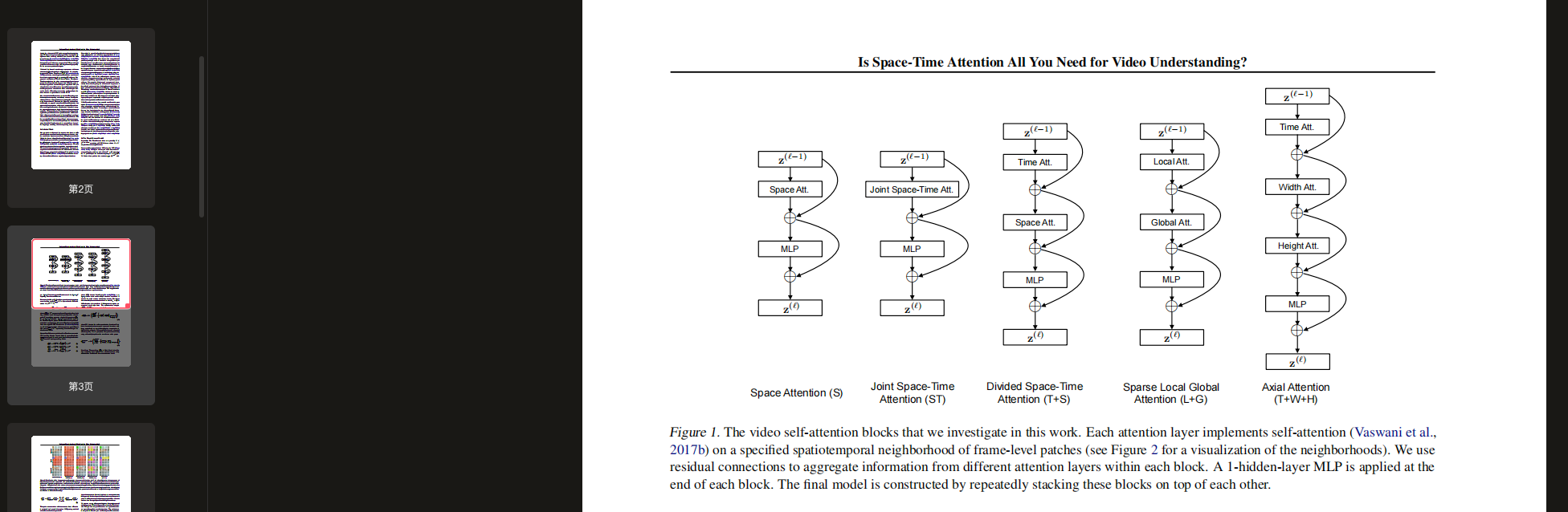
A. 段落分解和分析

逐句分析：

[句子1]

• 原文：Figure 1. The video self-attention blocks that we investigate in this work.

• 翻译：图1. 本研究中探究的视频自注意力模块。

• 解释：

  • 重点词汇：video self-attention blocks（视频自注意力模块）
  • 句子结构：简单句，图片标题
  • 与上下文关系：引入图1的主题
  • 难点解释：指出了图示内容的主要对象

[句子2]

• 原文：Each attention layer implements self-attention (Vaswani et al., 2017b) on a specified spatiotemporal neighborhood of frame-level patches (see Figure 2 for a visualization of the neighborhoods).

• 翻译：每个注意力层在指定的帧级patches的时空邻域上实现自注意力（Vaswani等，2017b）（参见图2中关于邻域的可视化）。

• 解释：

  • 重点词汇：attention layer（注意力层）, spatiotemporal neighborhood（时空邻域）
  • 句子结构：复合句，解释注意力层的工作机制
  • 与上下文关系：与图2建立连接，详细说明了模块的工作原理
  • 难点解释：说明了注意力计算的具体实现方式

[句子3]

• 原文：We use residual connections to aggregate information from different attention layers within each block.

• 翻译：我们使用残差连接来聚合每个模块中不同注意力层的信息。

• 解释：

  • 重点词汇：residual connections（残差连接）, aggregate information（聚合信息）
  • 句子结构：简单句，描述信息聚合方式
  • 与上下文关系：解释了模块内部的信息流动机制
  • 难点解释：说明了如何处理多层注意力的输出

[句子4]

• 原文：A 1-hidden-layer MLP is applied at the end of each block. The final model is constructed by repeatedly stacking these blocks on top of each other.

• 翻译：在每个模块的末端应用一个单隐层MLP。最终的模型通过将这些模块反复堆叠构建而成。

• 解释：

  • 重点词汇：1-hidden-layer MLP（单隐层MLP）, stacking（堆叠）
  • 句子结构：两个简单句，描述模型的最终构建方式
  • 与上下文关系：总结了模块的最后处理步骤和整体模型构建方法
  • 难点解释：阐明了单个模块的完整结构和模型的组织方式

B. 段落整体理解

段落主旨：

解释图1中展示的视频自注意力模块的架构和工作原理。

核心要点：

• 每个注意力层处理特定的时空邻域
• 使用残差连接整合多层信息
• 每个模块末端使用MLP处理
• 通过堆叠模块构建完整模型

与其他段落的关系：

本段作为图1的说明文字，提供了模型架构的具体细节，并与图2形成互补

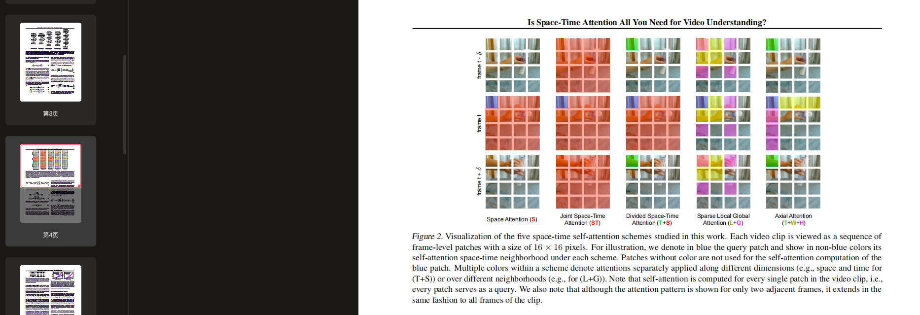
图2

A. 段落分解和分析

逐句分析：

[句子1]

• 原文：Figure 2. Visualization of the five space-time self-attention schemes studied in this work.

• 翻译：图2. 本研究中研究的五种时空自注意力方案的可视化。

• 解释：

  • 重点词汇：space-time self-attention schemes（时空自注意力方案）
  • 句子结构：简单句，图片标题
  • 与上下文关系：介绍了图2的主要内容
  • 难点解释：表明将展示不同的注意力计算方案

[句子2]

• 原文：Each video clip is viewed as a sequence of frame-level patches with a size of 16 × 16 pixels.

• 翻译：每个视频片段被视为一系列大小为16 × 16像素的帧级patches。

• 解释：

  • 重点词汇：video clip（视频片段）, frame-level patches（帧级patch）
  • 句子结构：简单句，描述基本数据处理单位
  • 与上下文关系：说明了数据预处理方式
  • 难点解释：定义了patch的具体大小和组织方式

[句子3]

• 原文：For illustration, we denote in blue the query patch and show in non-blue colors its self-attention space-time neighborhood under each scheme.

• 翻译：为了说明，我们用蓝色表示查询patch，用非蓝色显示在每种方案下的时空自注意力邻域。

• 解释：

  • 重点词汇：query patch（查询patch）, self-attention space-time neighborhood（时空自注意力邻域）
  • 句子结构：复合句，解释图示的颜色编码方式
  • 与上下文关系：解释图示的表示方法
  • 难点解释：说明了不同颜色的含义和用途

[句子4]

• 原文：Patches without color are not used for the self-attention computation of the blue patch. Multiple colors within a scheme denote attentions separately applied along different dimensions (e.g., space and time for (T+S)) or over different neighborhoods (e.g., for (L+G)).

• 翻译：无颜色的patches不用于蓝色patch的自注意力计算。方案中的多种颜色表示沿不同维度（例如(T+S)中的空间和时间维度）或在不同邻域（例如(L+G)）上分别应用的注意力。

• 解释：

  • 重点词汇：self-attention computation（自注意力计算）, dimensions（维度）, neighborhoods（邻域）
  • 句子结构：复合句，解释了颜色编码的详细含义
  • 与上下文关系：进一步详细说明了可视化方案的表示方法
  • 难点解释：区分了不同模型中颜色编码的不同含义

[句子5]

• 原文：Note that self-attention is computed for every single patch in the video clip, i.e., every patch serves as a query. We also note that although the attention pattern is shown for only two adjacent frames, it extends in the same fashion to all frames of the clip.

• 翻译：注意，自注意力是为视频片段中的每个单独patch计算的，即每个patch都作为查询patch。我们还需要注意，虽然注意力模式仅显示了两个相邻帧，但它以相同方式扩展到片段的所有帧。

• 解释：

  • 重点词汇：single patch（单独patch）, attention pattern（注意力模式）, adjacent frames（相邻帧）
  • 句子结构：复合句，提供了两个重要说明
  • 与上下文关系：补充说明了图示的泛化性
  • 难点解释：强调了注意力计算的全局性和模式的扩展性

B. 段落整体理解

段落主旨：

详细解释了图2中不同时空自注意力方案的可视化表示方法。

核心要点：

• 视频被分解为16×16像素的patches
• 使用颜色编码表示不同的注意力计算方案
• 每个patch都作为查询patch参与计算
• 注意力模式在时间维度上具有一致性

与其他段落的关系：

本段作为图2的说明文字，补充了前文对各种注意力模型的理论描述

C. 专业知识拓展

术语解释：

• Space-time self-attention：时空自注意力，在时间和空间维度上同时计算的注意力机制
• Frame-level patches：帧级patches，将视频帧分割成的小块
• Query patch：查询patch，当前计算注意力的目标patch
• Attention pattern：注意力模式，注意力计算的空间分布模式
• Adjacent frames：相邻帧，视频序列中连续的两帧

背景信息：

• 视频处理中需要同时考虑空间和时间维度的信息
• Patch是视频处理的基本单位

补充说明：

• 不同颜色编码反映了不同的注意力计算策略
• 模型设计考虑了计算效率和表示能力的平衡

表1

A. 段落分解和分析

逐句分析：

[句子1]

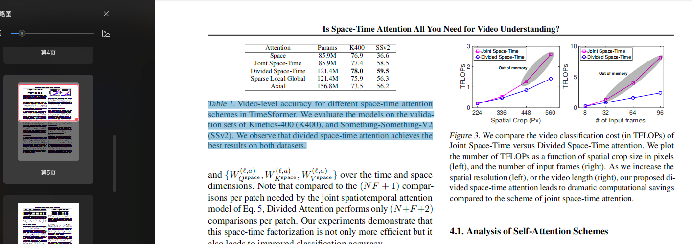
• 原文：Table 1. Video-level accuracy for different space-time attention schemes in TimeSformer.

• 翻译：表1. TimeSformer中不同时空注意力方案的视频级准确率。

• 解释：

  • 重点词汇：Video-level accuracy（视频级准确率）, space-time attention schemes（时空注意力方案）
  • 句子结构：简单句，表格标题
  • 与上下文关系：引入表格的主要内容
  • 难点解释：指出了表格展示的性能指标

[句子2]

• 原文：We evaluate the models on the validation sets of Kinetics-400 (K400), and Something-Something-V2 (SSv2).

• 翻译：我们在Kinetics-400（K400）和Something-Something-V2（SSv2）的验证集上评估这些模型。

• 解释：

  • 重点词汇：validation sets（验证集）
  • 句子结构：简单句，说明评估数据集
  • 与上下文关系：说明实验设置
  • 难点解释：指明了用于评估的具体数据集

[句子3]

• 原文：We observe that divided space-time attention achieves the best results on both datasets.

• 翻译：我们观察到分离的时空注意力在两个数据集上都取得了最好的结果。

• 解释：

  • 重点词汇：divided space-time attention（分离的时空注意力）
  • 句子结构：简单句，总结主要发现
  • 与上下文关系：给出实验结论
  • 难点解释：指出了性能最优的注意力方案

B. 内容整体理解

主要内容：

表1展示了不同时空注意力方案在两个主要视频数据集上的性能比较。

核心要点：

• 比较了TimeSformer中不同注意力方案
• 使用K400和SSv2两个数据集进行评估
• 分离的时空注意力方案表现最佳

实验设置：

• 评估指标：视频级准确率（video-level accuracy）
• 数据集：K400和SSv2验证集
• 模型：TimeSformer的不同变体

C. 专业知识拓展

术语解释：

• TimeSformer：基于Transformer架构的视频理解模型
• Kinetics-400：包含400个动作类别的大规模视频数据集
• Something-Something-V2：关注时序动作理解的视频数据集
• Divided space-time attention：将空间和时间维度分开处理的注意力机制

背景信息：

• 视频理解需要同时处理空间和时间信息
• 不同的注意力机制会影响模型性能
• 验证集用于评估模型的泛化能力

补充说明：

• 实验结果支持时空分离处理的有效性
• 结论在两个不同性质的数据集上都成立
• 为视频模型设计提供了指导