


参考 文章 和论文
http://www.jos.org.cn/html/2014/3/4410.htm#outline_anchor_8
KAIS_2004_warping.pdf
背景介绍:
Suppose we have two time series, Q and C, of length n and m, respectively, where
Q = q1, q2,. . ., qi,. . ., qn (1)
C = c1, c2,. . ., c j,. . ., cm. (2)
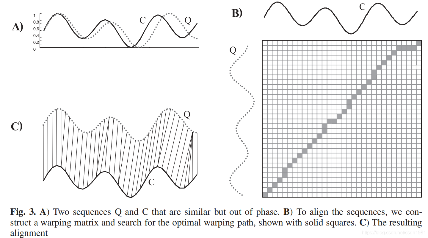
To align two sequences using DTW, we construct an n-by-m matrix where the
(ith, jth) element of the matrix contains the distance d(qi, cj) between the two points
qi and cj (i.e. d(qi, c j) = (qi − c j)2). Each matrix element (i, j) corresponds to
the alignment between the points qi and c j. This is illustrated in Fig. 3. A warping
path W is a contiguous (in the sense stated below) set of matrix elements that defines
a mapping between Q and C. The kth element of W is defined as wk = (i, j)k. So
Exact indexing of dynamic time warping
we have
W = w1,w2,. . .,wk,. . .,wK max(m, n) ≤ K < m + n − 1. (3)
The warping path is typically subject to several constraints.
采用 Q,C 代表2个时间序列的数据, 长度对应为 n 和 m, 构建 一个 n * m 的 矩阵 来表示, qi 和 cj 所代表的数据点 对应的 距离 d(qi,cj), 示意图 如下所示, 一个 代表 Q,C数据关联性的 扭曲路径 是一个 有着连续相连 矩阵 元素的 路径, 示意图 如 Fig3 的图 B 所示。
确切得可索引 动态时间 扭曲 路径 的定义 为如下 公式 (3) 所示。
W = w1,w2,. . .,wk,. . .,wK max(m, n) ≤ K < m + n − 1. (3)
 This path can be found using dynamic programming to evaluate the following Recurrence, which defines the cumulative distance γ(i, j) as the distance d(i, j) found
in the current cell and the minimum of the cumulative distances of the adjacent
elements:
γ(i, j) = d(qi, c j) + min {γ(i − 1, j − 1),γ(i − 1, j),γ(i, j − 1)}. (5)
这个相关时间扭曲 的路径 可以采用 动态 规划 方法 结合 前几个 的 可能性的路径 来计算, 定义
γ(i, j) 为 当前矩阵 小格 和 之前累计的临近小格(对应当前小格的左边,右边或者对角) 的 最小值 ,两者相加的和。
γ(i, j) = d(qi, c j) + min {γ(i − 1, j − 1),γ(i − 1, j),γ(i, j − 1)}. (5)
Lower bounding the DTW distance
DTW 的 下边界 距离 的 处理, 目前 有大概如下几种 对距离的 定义 和处理。
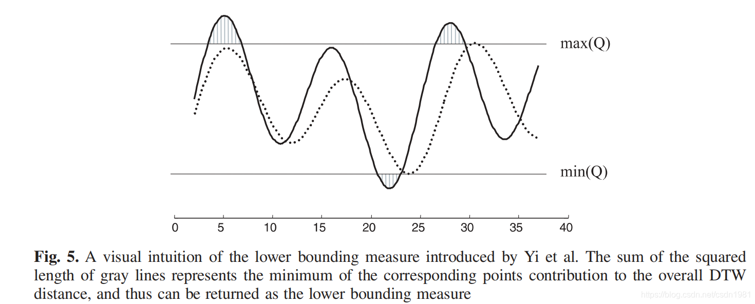
LB_Yi 示意图 如下。
计算两条一元时间序列的DTW下界距离时,选择一条序列作为基准序列,以另一条序列中大于基准序列最大值的点集以及小于基准序列最小值的点集作为特征,以此为基础构造DTW下界距离,记为LB_Yi
 LB_Kim 方案 的示意图 如下。
提取一元时间序列的起始点、结束点、最大值点和最小值点这4个特征,以此为基础构造DTW下界距离,记为LB_Kim
 论文 建议的 一种度量lower bouding (下边界距离)的方法。
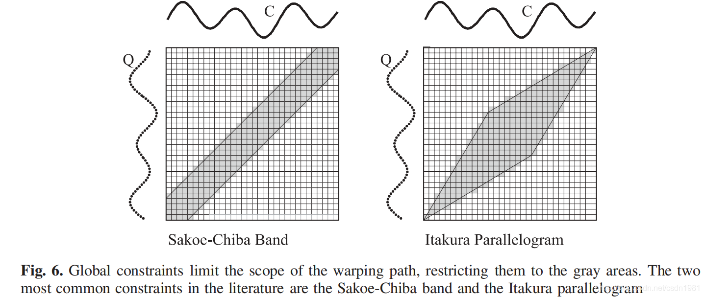
DTW 数据对比 扭曲 窗口 大小的 概念定义。两种定义方法, Chiba 和 Itakura 两种
目的是为了 定义 在 数据 对比上 一个 滑动窗口 的概念,防止 没必要的时间窗口上不相关数据的过度比较。这种称之 为 整体 限制 (global constraints).
The subset of the matrix
that the warping path is allowed to visit is called the warping window. Figure 6
illustrates two of the most frequently used global constraints, the Sakoe-Chiba band
(Sakoe and Chiba 1978) and the Itakura parallelogram (Itakura 1975).
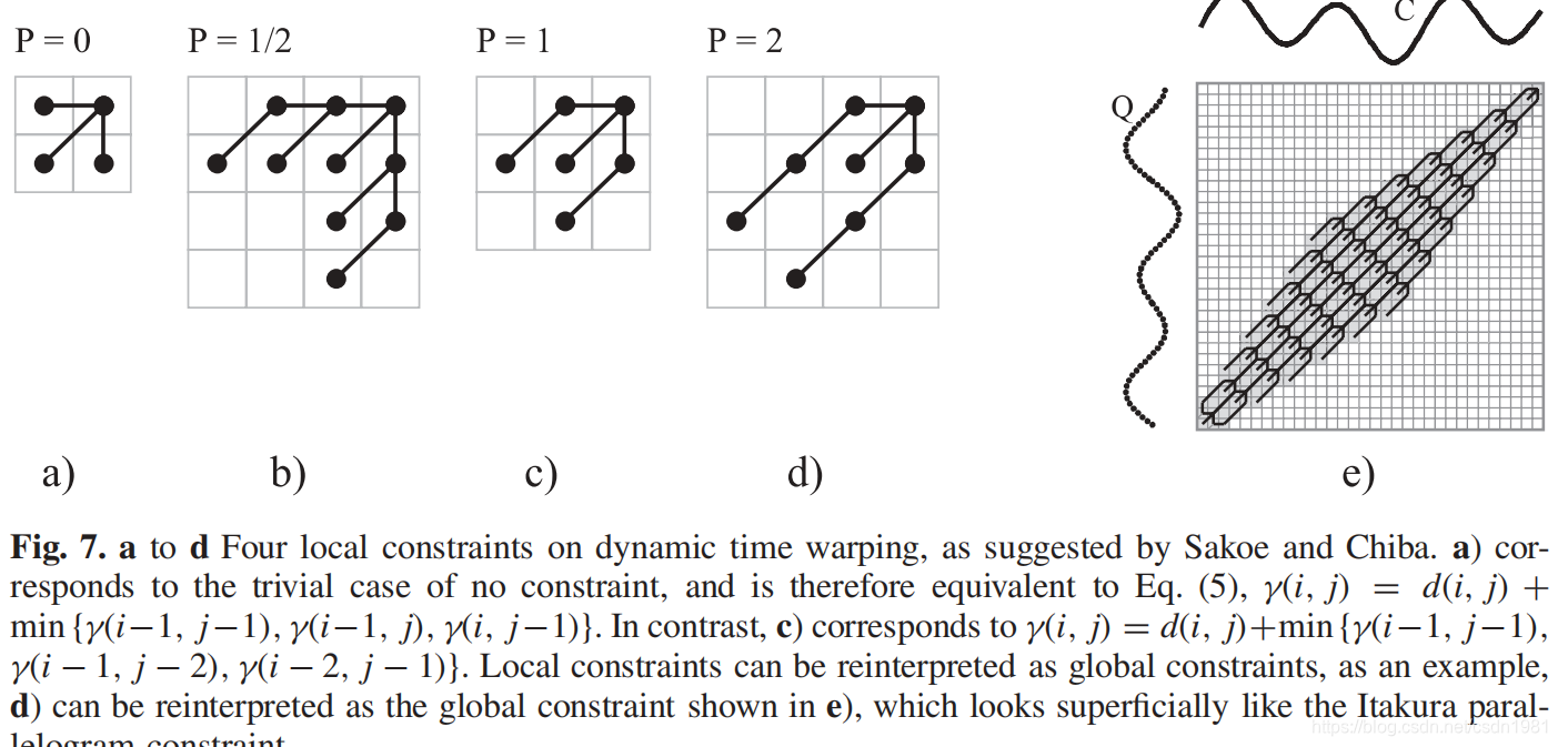
 针对 整体 限制 还有一个 称之为 局部 限制的方法, 示意图如下。
主要是 针对 DTW 对应点距离的 MIN 部分的 计算参考点往后或者 往左移动更多距离。也就是针对本文里面的公式 (5) 做的一些修正,这个修正主要还是依赖 采用该方法 的行业和数据来决定。
 下面是 论文建议的 lower bounding 的度量方法。
定义 一个 范围 r 来确定 bouding 的范围,
设一元查询序列Q=áq1,q2,…,qnñ,弯曲路径在全局约束条件下的弯曲限制为r,定义两条新序列U=áu1,u2,…, unñ,L=ál1,l2,…,lnñ:
ui=max(qi-r,qi+r) (6)
li=min(qi-r,qi+r) (7)
Q被包围在上、下边界序列形成的区域中,该区域称为封袋.
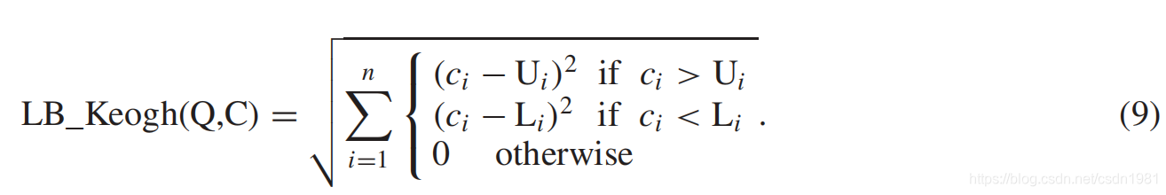
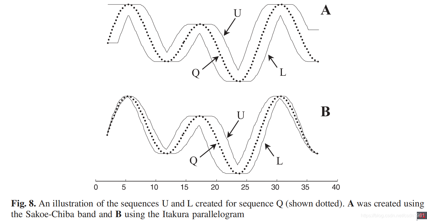 因此 LB_Keogh 的 大致定义 如下
很明显, qi 的 界定 范围 在 Ui Li 直接
∀i Ui ≥ qi ≥ Li. (8)


 被折叠的 条评论
为什么被折叠?
被折叠的 条评论
为什么被折叠?
 到【灌水乐园】发言


