谷歌浏览器表格无法导入_如何从另一个Google表格导入数据-CSDN博客

本文介绍了如何在Google Sheets中从另一个工作表或不同文档导入数据。你可以通过引用公式在同一个文档的不同工作表间导入数据，或者使用链接引用不同文档的单元格。导入时，如果遇到#REF!错误，只需允许访问即可。

摘要生成于 C知道，由 DeepSeek-R1 满血版支持，前往体验 >

谷歌浏览器表格无法导入

Should you need to import data from another spreadsheet in Google Sheets, you can do it a couple of ways. Whether you want to pull the data from another sheet in the file or an entirely different spreadsheet, here’s how.

如果您需要从Google表格中的另一个电子表格中导入数据，可以采用以下两种方法。无论您是要从文件中的另一个工作表中提取数据，还是要从完全不同的电子表格中提取数据，都是这样。

从另一个工作表导入数据 (Import Data from Another Sheet)

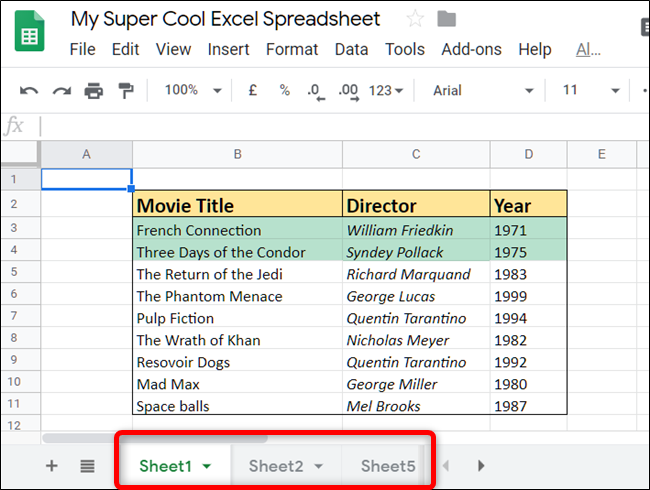
This first method requires you to have more than one sheet inside of a document. You can see whether your document has more than one sheet by looking at the bottom of the page. And to add another one, just hit the plus sign (+) to create a new one.

第一种方法要求您在一个文档中包含多个工作表。通过查看页面底部，可以查看文档是否有一张以上的纸。要添加另一个，只需点击加号(+)即可创建一个新的。

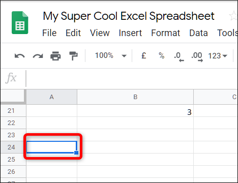
Multiple sheets inside of a document are located at the bottom of the page.

Fire up your browser, head to Google Sheets, and open up a spreadsheet. Click and highlight the cell where you want to import the data.

启动浏览器，转到Google表格，然后打开一个电子表格。单击并突出显示要在其中导入数据的单元格。

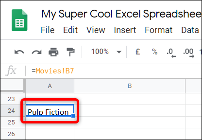
Click an empty cell where you want the data to go.

Next, you need to type in a formula that references the cell from the other sheet. If your sheets are named, you will want to put its name in place of <SheetName> and the cell you want to reference after the exclamation mark. It should look something like this:

接下来，您需要输入引用另一张工作表中的单元格的公式。如果您的工作表已命名，则将其名称替换为<SheetName>和要在感叹号后引用的单元格。它看起来应该像这样：

=<SheetName>!B7

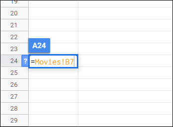
Type = followed by the name of the sheet and the cell you want to import.

Hit the “Enter” key and the data from the other sheet will show up in that cell.

按下“ Enter”键，另一个工作表中的数据将显示在该单元格中。

Like magic, the cell gets populated with the data.

从另一个文档导入数据 (Import Data from Another Document)

In addition to importing data from a sheet within a spreadsheet, you can reference cell(s) from a completely different document. The formula is slightly modified from the previous one but works almost identically.

除了从电子表格中的工作表中导入数据之外，您还可以引用完全不同的文档中的单元格。该公式与前一个公式稍作修改，但几乎相同。

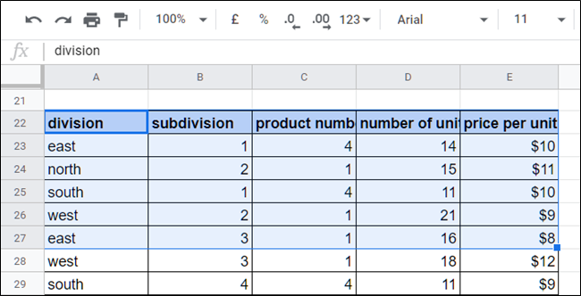
Fire up the document you want to import data from and write down the range of cells to reference. For this guide, we want the range A22:E27.

启动要从中导入数据的文档，并写下要引用的单元格范围。对于本指南，我们需要范围A22：E27。

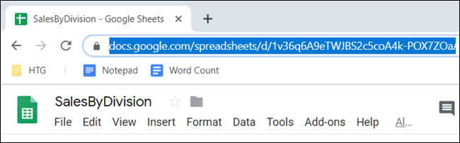
Write down the cell range you want to import. We are using A22:E27 for this guide.

Next, copy the complete URL of the spreadsheet to the clipboard. Click the address bar, and then use the keyboard shortcut Ctrl+C (Windows/Chrome OS) or Cmd+C (macOS).

接下来，将电子表格的完整URL复制到剪贴板。单击地址栏，然后使用键盘快捷键 Ctrl + C(Windows / Chrome OS)或Cmd + C(macOS)。

Select and copy the URL to your clipboard.

Now, head back to the Google Sheets home page and open the spreadsheet where you want to import the data.

现在，返回Google表格首页，然后打开要在其中导入数据的电子表格。

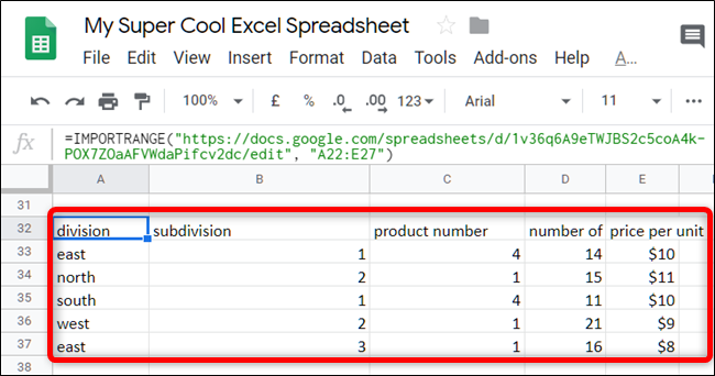
Click on an empty cell and type =IMPORTRANGE("<URL>" , "<CellRange>") , where <URL> is the link you copied and <CellRange> denotes the cells you want to import that you wrote down. Paste the URL between the quotation marks by pressing Ctrl+V (Windows/Chrome OS) or Cmd+V (macOS), type in the range, and then hit Enter. It should look like this:

单击一个空单元格，然后键入=IMPORTRANGE("<URL>" , "<CellRange>") ，其中<URL>是您复制的链接，而<CellRange>表示您要记下的要导入的单元格。通过按Ctrl + V(Windows / Chrome OS)或Cmd + V(macOS)将URL粘贴在引号之间，键入范围，然后按Enter。它看起来应该像这样：

=IMPORTRANGE("http://docs.google.com/spreadsheets/d/URL/to/spreadsheet/edit" , "A22:E27")

Note: If you have more than one sheet in the other document, you must specify which one you want to reference. For example, if you’re importing from Sheet2, you would type “Sheet2!A22:E27” instead.

注意：如果另一文档中有多个工作表，则必须指定要引用的工作表。例如，如果要从Sheet2导入，则应键入“ Sheet2！A22：E27”。

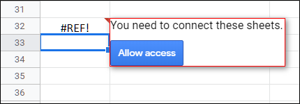
Hit Enter and you should see the error “#REF!”. This is normal, Google Sheets just needs you to allow it access to the other sheet. Select the cell with the error and then click “Allow Access.”

按下Enter键，您应该看到错误“ #REF！”。这很正常，Google表格仅需要您允许其访问其他表格。选择出现错误的单元格，然后单击“允许访问”。

Allow your spreadsheet to access the other one and click "Allow Access."

It should take a couple of seconds to load, but when it’s finished, the data range will import everything directly into your spreadsheet.

加载需要花费几秒钟的时间，但是完成后，数据范围会将所有内容直接导入到电子表格中。

Again, like magic, all the data from the range of cells is imported into your document.

Although cell formatting—such as colors—doesn’t follow data over when importing from other sheets, these are the best ways to reference external cells in Google Sheets.

虽然单元格格式(例如颜色)在从其他工作表导入时不会遵循数据，但是这些是引用Google表格中外部单元格的最佳方法。