


Previously, in this Data science series, I already tacitly did quite a few aggregations over the whole dataset and aggregations over groups of data. Of course, the vast majority of the readers here is familiar with the GROUP BY clause in the T-SQL SELECT statement and with the basic aggregate functions. Therefore, in this article, I want to show some advanced aggregation options in T-SQL and grouping in aggregations of data in an R or a Python data frame.
以前,在本数据科学系列中,我已经默认对整个数据集和数据组进行了很多聚合。 当然,这里的绝大多数读者都熟悉T-SQL SELECT语句中的GROUP BY子句以及基本的聚合函数。 因此,在本文中,我想显示T-SQL中的一些高级聚合选项,以及在R或Python数据帧中的数据聚合中进行分组。
Aggregating data might be a part of data preparation in data science, a part of data overview, or even already a part of the finaly analysis of the data.
聚合数据可能是数据科学中数据准备的一部分,数据概述的一部分,甚至已经是数据最终分析的一部分。
T-SQL分组集 (T-SQL Grouping Sets)
The T-SQL language does not have a plethora of different aggregate functions. However, you can do a lot of different ways of grouping of the same rows with just a few lines of code in T-SQL.
T-SQL语言没有太多不同的聚合函数。 但是,在T-SQL中只需几行代码,您就可以采用多种不同的方式对同一行进行分组。
Let me start with the basic aggregation over groups in T-SQL. The following code calculates the number of customers per country ordered by the country name, using the COUNT(*) aggregate function. You define the grouping variables in the GROUP BY clause.
让我从T-SQL中的组的基本聚合开始。 以下代码使用COUNT(*)聚合函数计算按国家/地区名称订购的每个国家/地区的客户数量。 您可以在GROUP BY子句中定义分组变量。
USE AdventureWorksDW2016;
SELECT g.EnglishCountryRegionName AS Country,
 COUNT(*) AS CustomersInCountry
FROM dbo.DimCustomer AS c
 INNER JOIN dbo.DimGeography AS g
  ON c.GeographyKey = g.GeographyKey
GROUP BY g.EnglishCountryRegionName
ORDER BY g.EnglishCountryRegionName;
The next step is to filter the results on the aggregated values. You can do this with the HAVING clause, like the following query shows. The query keeps in the result only the countries where there are more than 3,000 customers.
下一步是根据合计值过滤结果。 您可以使用HAVING子句执行此操作,如以下查询所示。 该查询仅保留结果中有3,000多个客户的国家/地区。
SELECT g.EnglishCountryRegionName AS Country,
 COUNT(*) AS CustomersInCountry
FROM dbo.DimCustomer AS c
 INNER JOIN dbo.DimGeography AS g
  ON c.GeographyKey = g.GeographyKey
GROUP BY g.EnglishCountryRegionName
HAVING COUNT(*) > 3000
ORDER BY g.EnglishCountryRegionName;
Besides ordering on the grouping expression, you can also order on the aggregated value, like you can see in the following query, which orders descending the states from different countries by the average income.
除了对分组表达式进行排序之外,您还可以对汇总值进行排序,就像在下面的查询中看到的那样,该排序以平均收入从不同国家/地区降序排列。
SELECT g.EnglishCountryRegionName AS Country,
 g.StateProvinceName AS State,
 AVG(c.YearlyIncome) AS AvgIncome
FROM dbo.DimCustomer AS c
 INNER JOIN dbo.DimGeography AS g
  ON c.GeographyKey = g.GeographyKey
GROUP BY g.EnglishCountryRegionName,
 g.StateProvinceName
ORDER BY AvgIncome DESC;
I guess there was not much new info in the previous examples for the vast majority of SQL Server developers. However, there is an advanced option of grouping in T-SQL that is not so widely known. You can perform many different ways of grouping in a single query with the GROUPING SETS clause. In this clause, you define different grouping variables in every single set. You could do something similar by using multiple SELECT statements with a single GROUP BY clause and then by unioning the results of them all. Having an option to do this in a single statement gives you the opportunity to make a lot of different grouping with only a few lines of code. In addition, this syntax enables SQL Server to better optimize the query. Look at the following example:
我想在前面的示例中,对于绝大多数SQL Server开发人员来说,没有太多新信息。 但是,在T-SQL中有一个分组的高级选项,尚不为人所知。 您可以使用GROUPING SETS子句在单个查询中执行多种不同的分组方式。 在此子句中,您在每个集合中定义了不同的分组变量。 您可以通过将多个SELECT语句与单个GROUP BY子句一起使用,然后将所有结果合并在一起,来执行类似的操作。 可以在单个语句中执行此操作,这使您有机会仅用几行代码就可以进行许多不同的分组。 此外,此语法使SQL Server可以更好地优化查询。 看下面的例子:
SELECT g.EnglishCountryRegionName AS Country,
 GROUPING(g.EnglishCountryRegionName) AS CountryGrouping,
 c.EnglishEducation AS Education,
 GROUPING(c.EnglishEducation) AS EducationGrouping,
 STDEV(c.YearlyIncome) / AVG(c.YearlyIncome)
  AS CVIncome
FROM dbo.DimCustomer AS c
 INNER JOIN dbo.DimGeography AS g
  ON c.GeographyKey = g.GeographyKey
GROUP BY GROUPING SETS
(
 (g.EnglishCountryRegionName, c.EnglishEducation),
 (g.EnglishCountryRegionName),
 (c.EnglishEducation),
 ()
)
ORDER BY NEWID();
The query calculates the coefficient of variation (defined as the standard deviation divided the mean) for the following groups, in the order as they are listed in the GROUPING SETS clause:
该查询按以下分组(在GROUPING SETS子句中列出的顺序)计算以下各组的变异系数(定义为标准偏差除以平均值):
- Country and education – expression (g.EnglishCountryRegionName, c.EnglishEducation) 国家和教育–表达式(g.EnglishCountryRegionName,c.EnglishEducation)
- Country only – expression (g.EnglishCountryRegionName) 仅国家/地区–表达式(g.EnglishCountryRegionName)
- Education only – expression (c.EnglishEducation) 仅限教育–表达(c.EnglishEducation)
- Over all dataset- expression () 遍及所有数据集表达式()
Note also the usage of the GROUPING() function in the query. This function tells you whether the NULL in a cell comes because there were NULLs in the source data and this means a group NULL, or there is a NULL in the cell because this is a hyper aggregate. For example, NULL in the Education column where the value of the GROUPING(Education) equals to 1 indicates that this is aggregated in such a way that education makes no sense in the context, for example, aggregated over countries only, or over the whole dataset. I used ordering by NEWID() just to shuffle the results. I executed query multiple times before I got the desired order where all possibilities for the GROUPING() function output were included in the first few rows of the result set. Here is the result.
还要注意查询中GROUPING()函数的用法。 此函数告诉您单元格中是否存在NULL是因为源数据中存在NULL,这意味着组NULL,还是单元格中存在NULL,因为这是超聚合。 例如,GROUPING(Education)的值等于1的“教育”列中的NULL表示这是以某种方式在上下文中没有意义的教育进行汇总的,例如,仅汇总到各个国家或整个汇总数据集。 我使用按NEWID()排序只是为了乱序结果。 在获得所需顺序之前,我多次执行查询,在该顺序中,GROUPING()函数输出的所有可能性都包含在结果集的前几行中。 这是结果。
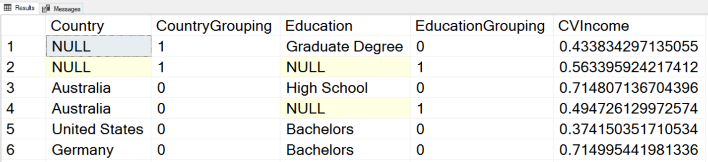
In the first row, you can see that Country is NULL, so this is an aggregate over Education only. In the second row, you can see that both Country and Education are NULL, meaning that this is an aggregate over the whole dataset. I will leave you to interpret the other results by yourself.
在第一行中,您可以看到Country为NULL,因此这仅是Education的汇总。 在第二行中,您可以看到Country和Education均为NULL,这意味着这是整个数据集的汇总。 我将让您自己解释其他结果。
在R中聚合 (Aggregating in R)
As you can imagine, there are countless possibilities for aggregating the data in R. In this data science article, I will show you only the options from the base installation, without any additional package. Let me start by reading the data from SQL Server.
可以想象,在R中聚合数据的可能性无数。在此数据科学文章中,我将仅向您展示基本安装中的选项,而无需任何其他软件包。 首先让我从SQL Server读取数据。
library(RODBC)
con <- odbcConnect("AWDW", uid = "RUser", pwd = "Pa$$w0rd")
TM <- as.data.frame(sqlQuery(con,
  "SELECT g.EnglishCountryRegionName AS Country,
    c.EnglishEducation AS Education,
    c.YearlyIncome AS Income
   FROM dbo.DimCustomer AS c
    INNER JOIN dbo.DimGeography AS g
     ON c.GeographyKey = g.GeographyKey;"),
  stringsAsFactors = TRUE)
close(con)
The first function I want to mention is the summarize() function. It is the simplest way of getting the basic descriptive statistics for a variable, or even for a complete data frame. In the following example, I am analyzing the Income and the Education variables from the TM data frame.
我要提到的第一个函数是summary()函数。 这是获取变量甚至整个数据帧的基本描述统计信息的最简单方法。 在下面的示例中,我正在分析TM数据框中的收入和教育变量。
summary(TM$Income)
摘要(TM $收入)
summary(TM$Education)
摘要(TM $教育)
Here are the results.
这是结果。
| Min. | 1st Qu. | Median | Mean | 3rd Qu. | Max. |
| 10000 | 30000 | 60000 | 57310 | 70000 | 170000 |
| Bachelors | Graduate Degree | High School | |||
| 5356 | 3189 | 3294 | |||
| Partial College | Partial High School | ||||
| 5064 | 1581 |
| 最小 | 第一区 | 中位数 | 意思 | 第三区 | 最高 |
| 10000 | 30000 | 60000 | 57310 | 70000 | 170000 |
| 学士学位 | 研究生学历 | 中学 | |||
| 5356 | 3189 | 3294 | |||
| 部分大学 | 偏高中 | ||||
| 5064 | 1581 |
You can see that the summary() function returned for a continuous variable the minimal and the maximal values, the values on the first and on the third quartile, and the mean and the median. For a factor, the function returned the absolute frequencies.
您可以看到summary()函数为连续变量返回了最小值和最大值,第一个和第三个四分位数上的值以及均值和中位数。 作为一个因素,该函数返回了绝对频率。
There are many other descriptive statistics functions already in base R. The following code shows quite a few of them by analyzing the Income variable.
基数R中已经有许多其他描述性统计函数。下面的代码通过分析Income变量显示了其中很多。
cat('  ','Mean  :', mean(TM$Income))
cat('\n','Median:', median(TM$Income))
cat('\n','Min   :', min(TM$Income))
cat('\n','Max   :', max(TM$Income))
cat('\n','Range :', range(TM$Income))
cat('\n','IQR   :', IQR(TM$Income))
cat('\n','Var   :', var(TM$Income))
cat('\n','StDev :', sd(TM$Income))
The code uses the cat() function which concatenates and prints the parameters. In the result, you can se the mean, the median, the minimal and the maximal value, the range and the inter-quartile range, and the variance and the standard deviation for the Income variable. Here are the results.
该代码使用cat()函数来串联并打印参数。 结果是,您可以设置平均值,中位数,最小值和最大值,范围和四分位间距以及收入变量的方差和标准差。 这是结果。
| Mean : | 57305.78 |
| Median: | 60000 |
| Min : | 10000 |
| Max : | 170000 |
| Range : | 10000 170000 |
| IQR : | 40000 |
| Var : | 1042375574 |
| StDev : | 32285.84 |
| 意思 : | 57305.78 |
| 中位数: | 60000 |
| 最小: | 10000 |
| 最大值: | 170000 |
| 范围 : | 10000 170000 |
| IQR: | 40000 |
| Var: | 1042375574 |
| 标准差: | 32285.84 |
You can use the aggregate() function to aggregate data over groups. Note the three parameters in the following example. The first one is the variable to be aggregated, the second is a list of variables used for grouping, and the third is the aggregate function. In the following example, I am calculating the sum of the income over countries.
您可以使用aggregate()函数来汇总组中的数据。 请注意以下示例中的三个参数。 第一个是要聚合的变量,第二个是用于分组的变量列表,第三个是聚合函数。 在以下示例中,我正在计算国家/地区的收入总和。
aggregate(TM$Income, by = list(TM$Country), FUN = sum)
As mentioned, the second parameter is a list of variables used to define the grouping. Let me show you an example with two variables in the list by calculating the mean value for the income over countries and education.
如前所述,第二个参数是用于定义分组的变量列表。 让我向您展示一个示例,其中通过计算国家和教育收入的平均值,列出了两个变量。
aggregate(TM$Income,
    by = list(TM$Country, TM$Education),
    FUN = mean)
The third parameter is the name of the function. This could also be a custom function. There is no built-in function in the base R installation for calculating the third and the fourth population moments, the skewness and the kurtosis. No problem, it is very easy to write a custom function. The following code shows the function, and then calculates the skewness and the kurtosis for the Income variable over the whole dataset and per country.
第三个参数是函数的名称。 这也可以是自定义函数。 基本R安装中没有内置函数来计算第三和第四人口矩,偏度和峰度。 没问题,编写自定义函数非常容易。 以下代码显示了该函数,然后计算整个数据集和每个国家/地区的Income变量的偏度和峰度。
skewkurt <- function(p) {
    avg <- mean(p)
    cnt <- length(p)
    stdev <- sd(p)
    skew <- sum((p - avg) ^ 3 / stdev ^ 3) / cnt
    kurt <- sum((p - avg) ^ 4 / stdev ^ 4) / cnt - 3
    return(c(skewness = skew, kurtosis = kurt))
};
skewkurt(TM$Income);
# Aggregations in groups with a custom function
aggregate(TM$Income, by = list(TM$Country), FUN = skewkurt)
Here are the results.
这是结果。
| skewness | kurtosis | ||
| 0.8219881 | 0.6451128 | ||
| Group.1 | x.skewness | x.kurtosis | |
| 1 | Australia | -0.05017649 | -0.50240998 |
| 2 | Canada | 0.95311355 | 3.19841011 |
| 3 | France | 1.32590706 | 0.56945630 |
| 4 | Germany | 1.32940136 | 0.35521164 |
| 5 | United Kingdom | 1.34856013 | 0.27294523 |
| 6 | United States | 1.17370389 | 2.08329296 |
| 偏度 | 峰度 | ||
| 0.8219881 | 0.6451128 | ||
| 第一组 | 偏度 | 峰度 | |
| 1个 | 澳大利亚 | -0.05017649 | -0.50240998 |
| 2 | 加拿大 | 0.95311355 | 3.19841011 |
| 3 | 法国 | 1.32590706 | 0.56945630 |
| 4 | 德国 | 1.32940136 | 0.35521164 |
| 5 | 英国 | 1.34856013 | 0.27294523 |
| 6 | 美国 | 1.17370389 | 2.08329296 |
If you need to filter the dataset on the aggregated values, you can store the result of the aggregation in a new data frame, and then filter the new data frame, like the following code shows.
如果需要根据聚合值过滤数据集,则可以将聚合结果存储在新数据框中,然后过滤新数据框,如以下代码所示。
TMAGG <- aggregate(list(Income = TM$Income),
    by = list(Country = TM$Country), FUN = mean)
TMAGG[TMAGG$Income > 60000,]
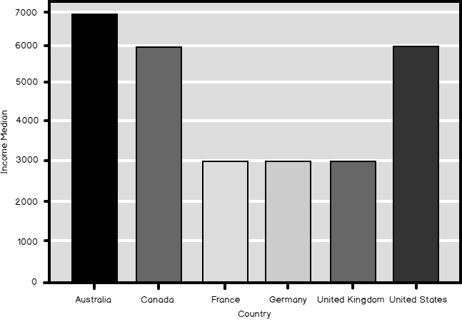
Finally, many of the graphical functions do the grouping and the aggregation by themselves. The barplot() function in the following example plots the bars showing the mean value of the income in each country.
最后,许多图形功能自行完成分组和聚合。 以下示例中的barplot()函数绘制了显示每个国家收入平均值的条形图。
barplot(TMAGG$Income,
    legend = TMAGG$Country,
    col = c('blue', 'yellow', 'red', 'green', 'magenta', 'black'))
The result is the following graph.
结果如下图。
Python Pandas聚合 (Python Pandas Aggregations)
As I explained in my previous article, in Python you get the data frame object when you load the pandas library. This library has also all of the methods you need to aggregate and groups the data and to create simple graphs. The following code imports the necessary libraries and reads the data from SQL Server.
正如我在上一篇文章中所解释的那样,在Python中,当您加载熊猫库时会获得数据框对象。 该库还具有汇总和分组数据以及创建简单图形所需的所有方法。 以下代码导入必要的库,并从SQL Server读取数据。
# Imports needed
import numpy as np
import pandas as pd
import pyodbc
import matplotlib.pyplot as plt
# Connecting and reading the data
con = pyodbc.connect('DSN=AWDW;UID=RUser;PWD=Pa$$w0rd')
query = """
SELECT g.EnglishCountryRegionName AS Country,
 c.EnglishEducation AS Education,
 c.YearlyIncome AS Income
FROM dbo.DimCustomer AS c
 INNER JOIN dbo.DimGeography AS g
  ON c.GeographyKey = g.GeographyKey;"""
TM = pd.read_sql(query, con)
The pandas data frame describe() method is quite similar to the R summary() function – provides you a quick overview of a variable. Besides this function, there are many separate descriptive statistics functions implemented as data frame methods as well. The list of these functions includes the functions that calculate the skewness and the kurtosis, as you can see from the following code.
大熊猫数据框的describe()方法与R summary()函数非常相似–为您提供了变量的快速概览。 除此功能外,还有许多单独的描述性统计功能也已实现为数据框方法。 这些功能的列表包括计算偏度和峰度的功能,如下面的代码所示。
# Summary
TM.describe()
# Count and variance
TM['Income'].count(), TM['Income'].var()
# Skewness and kurtosis
TM['Income'].skew(), TM['Income'].kurt()
Here are the results – descriptive statistics for the Income variable. You should be able to interpret the results by yourself without any problem.
这是结果–收入变量的描述性统计数据。 您应该能够自行解释结果。
>>> # Summary
              Income
count   18484.000000
mean    57305.777970
std     32285.841703
min     10000.000000
25%     30000.000000
50%     60000.000000
75%     70000.000000
max    170000.000000
>>> # Count and variance
 (18484, 1042375574.4691552)
>>> # Skewness and kurtosis
 (0.82212157713655321, 0.64600652578292239)
The pandas data frame groupby() method allows you to calculate the aggregates over groups. You can see in the following example calculation of counts, medians, and descriptive statistics of the Income variable over countries.
熊猫数据框groupby()方法允许您计算各组的聚合。 您可以在以下示例中查看国家/地区收入变量的计数,中位数和描述性统计的计算。
TM.groupby('Country')['Income'].count()
TM.groupby('Country')['Income'].median()
TM.groupby('Country')['Income'].describe()
For the sake of brevity, I am showing only the counts here.
为了简洁起见,我仅在此处显示计数。
| Country | |
| Australia | 3591 |
| Canada | 1571 |
| France | 1810 |
| Germany | 1780 |
| United Kingdom | 1913 |
| United States | 7819 |
| 国家 | |
| 澳大利亚 | 3591 |
| 加拿大 | 1571 |
| 法国 | 1810 |
| 德国 | 1780年 |
| 英国 | 1913年 |
| 美国 | 7819 |
If you need to filter the dataset based on the aggregated values, you can do it in the same way as in R. You store the results in a new data frame, and then filter the new data frame, like the following code shows.
如果需要基于聚合值过滤数据集,则可以按照与R中相同的方式进行。将结果存储在新数据框中,然后过滤新数据框,如以下代码所示。
TMAGG = pd.DataFrame(TM.groupby('Country')['Income'].median())
TMAGG.loc[TMAGG.Income > 50000]
Like the R graphing functions also the pandas data frame plot() function groups the data for you. The following code generates a bar chart with the medain income per country.
像R绘图函数一样,pandas数据框plot()函数也为您分组数据。 以下代码生成一个条形图,其中包含每个国家/地区的普通收入。
ax = TMAGG.plot(kind = 'bar',
           colors = ('b', 'y', 'r', 'g', 'm', 'k'),
           fontsize = 14, legend = False,
           use_index = True, rot = 1)
ax.set_xlabel('Country', fontsize = 16)
ax.set_ylabel('Income Median', fontsize = 16)
plt.show()
And here is the bar chart as the final result of the code in this data science article. Compare the median and the mean (shown in the graph created with the R code) of the Income in different countries.
这是此数据科学文章中代码最终结果的条形图。 比较不同国家/地区的收入中位数和均值(在使用R代码创建的图形中显示)。
结论 (Conclusion)
I am not done with grouping and aggregating in this series of Data science articles yet. In the following article, I plan to show you some advanced examples of GROUPING SETS clause in T-SQL. I will show you how to use some efficient grouping and aggregating methods in R by using external packages. I will do an additional deep dive in pandas data frame options for grouping and aggregating data.
在这一系列的数据科学文章中,我还没有完成分组和聚合的工作。 在下面的文章中,我计划向您展示T-SQL中GROUPING SETS子句的一些高级示例。 我将向您展示如何通过使用外部包在R中使用一些有效的分组和聚合方法。 我将对pandas数据框选项进行进一步的深入研究,以对数据进行分组和汇总。
目录 (Table of contents)
参考资料 (References)
- AggregatFunctions (Transact-SQL) in Microsoft Docs Microsoft Docs中的AggregatFunctionFunctions(Transact-SQL)
- SELECT – GROUP BY (Transact-SQL) in Microsoft Docs SELECT – Microsoft Docs中的GROUP BY(Transact-SQL)
- GROUPING (Transact-SQL) in Microsoft Docs Microsoft Docs中的分组(Transact-SQL)
- R summary function R汇总功能
- Concatenate and print – cat R function 连接和打印– cat R功能
- Compute summary statistics of data subsets – aggregate in R 计算数据子集的摘要统计信息-R中的汇总
- Skewness and kurtosis in the NIST / SEMATECH统计方法电子手册中的 NIST/SEMATECH e-Handbook of Statistical Methods 偏度和峰度
- The pandas data frame describe() function 熊猫数据框describe()函数
- The pandas data frame groupby() function 熊猫数据框groupby()函数


 3515
3515

 被折叠的 条评论
为什么被折叠?
被折叠的 条评论
为什么被折叠?
 到【灌水乐园】发言


